From GPT-2 to Kimi K3, from first principles
How a Transformer’s growing filing cabinet became a hybrid of editable memory, global token access, sparse specialists, and access to earlier thought.
Kimi K3 can look like an intimidating bag of acronyms: KDA, MLA, AttnRes, MoE, SiTU-GLU, QB, Muon, MXFP4. Read that list in isolation and it feels as if the Transformer has been replaced by something unrecognizable.
It has not.
Kimi K3 is still a causal, next-token-predicting decoder. Tokens become vectors. Layers mix information across token positions and across feature channels. A language-model head scores the next token. Training still adjusts parameters to make observed continuations more likely.
What changed is the machinery used to move information through three dimensions:
- Across sequence: Kimi Delta Attention carries a fixed-size, editable running memory; periodic Multi-head Latent Attention layers retain global softmax access to token-level history.
- Across width: Stable LatentMoE routes each token through a small subset of a very large expert pool.
- Across depth: Attention Residuals let later layers select useful earlier representations instead of accepting one uniformly accumulated residual stream.
The complete model adds a fourth story: images and videos enter through a vision encoder trained jointly with the language backbone from the beginning. Then pre-training, agentic reinforcement learning, quantization-aware post-training, and an unusually elaborate serving system turn the architecture into a deployed model.
This book builds those ideas in the order in which they become necessary. The goal is not to memorize the K3 diagram. It is to reach the point where you could have anticipated its major components from the failure modes of the previous design.
Prerequisite: This assumes you know embeddings, matrix multiplication, activation functions, backpropagation, and the ordinary Transformer block. If query/key/value attention or the residual stream still feels slippery, read Inside a Transformer, Slowly first. It deliberately ends where this book begins.
Before we begin
What “from first principles” means here
We will not re-teach neural networks from zero. We will repeatedly do four more useful things:
- state the object being computed and its tensor shape;
- identify the bottleneck that motivates the next design;
- work one small numerical example before returning to K3 scale;
- separate what a source establishes from the intuition we use to remember it.
Throughout the book, labels have a specific meaning:
- Evidence: a claim stated in the released K3 report, configuration, implementation, or an antecedent paper.
- Derived: arithmetic or a consequence calculated from those released quantities.
- Intuition: a useful mental model, not a literal description of learned representations.
That distinction matters. “KDA is an editable whiteboard” is good intuition. “KDA stores one symbolic fact in each row” would be a false architectural claim.
The fast path
If you already know ordinary attention well, read Chapters 0, 2–10, and 15. Chapters 11–14 explain why the final model is more than its backbone: native multimodal pre-training, post-training, and systems co-design are central to the result.
The whole argument in seven sentences
Full attention preserves a separate key and value for every token, providing sharp retrieval at a cost that grows with context. Linear attention compresses prior key-value associations into a fixed-size matrix, improving efficiency but introducing interference. DeltaNet treats that matrix as fast weights and writes prediction errors, allowing targeted replacement. Gated DeltaNet adds a global memory-retention control. Kimi Delta Attention gives different key channels different retention rates and changes the gate parameterization so chunkwise computation maps well to Tensor Cores. Because any fixed-size state must lose some detail, K3 interleaves three KDA layers with one global MLA layer. Stable LatentMoE and Attention Residuals then scale conditional width and selective depth access, while native vision, pre-training, RL, quantization, and serving infrastructure make the complete K3 system.
0. The model in one picture
The released K3 backbone is easiest to orient by separating the execution order inside a layer from the two schedules across layers:
text embeddings ---------+
                         +--> shared input representation
MoonViT-V2 -> projector --+

every decoder layer l:

depth sources -> AttnRes #1 -> attention input
attention input -> KDA or Gated MLA -> update depth state

updated depth sources -> AttnRes #2 -> feed-forward input
feed-forward input -> dense SiTU-GLU if l = 1
                   -> Stable LatentMoE if l = 2...93
                   -> update depth state
Figure 1. Each decoder layer performs two separate depth-retrieval steps: one before token mixing and one before channel mixing. The schedule below shows which token and channel mixers appear across the 93 layers.
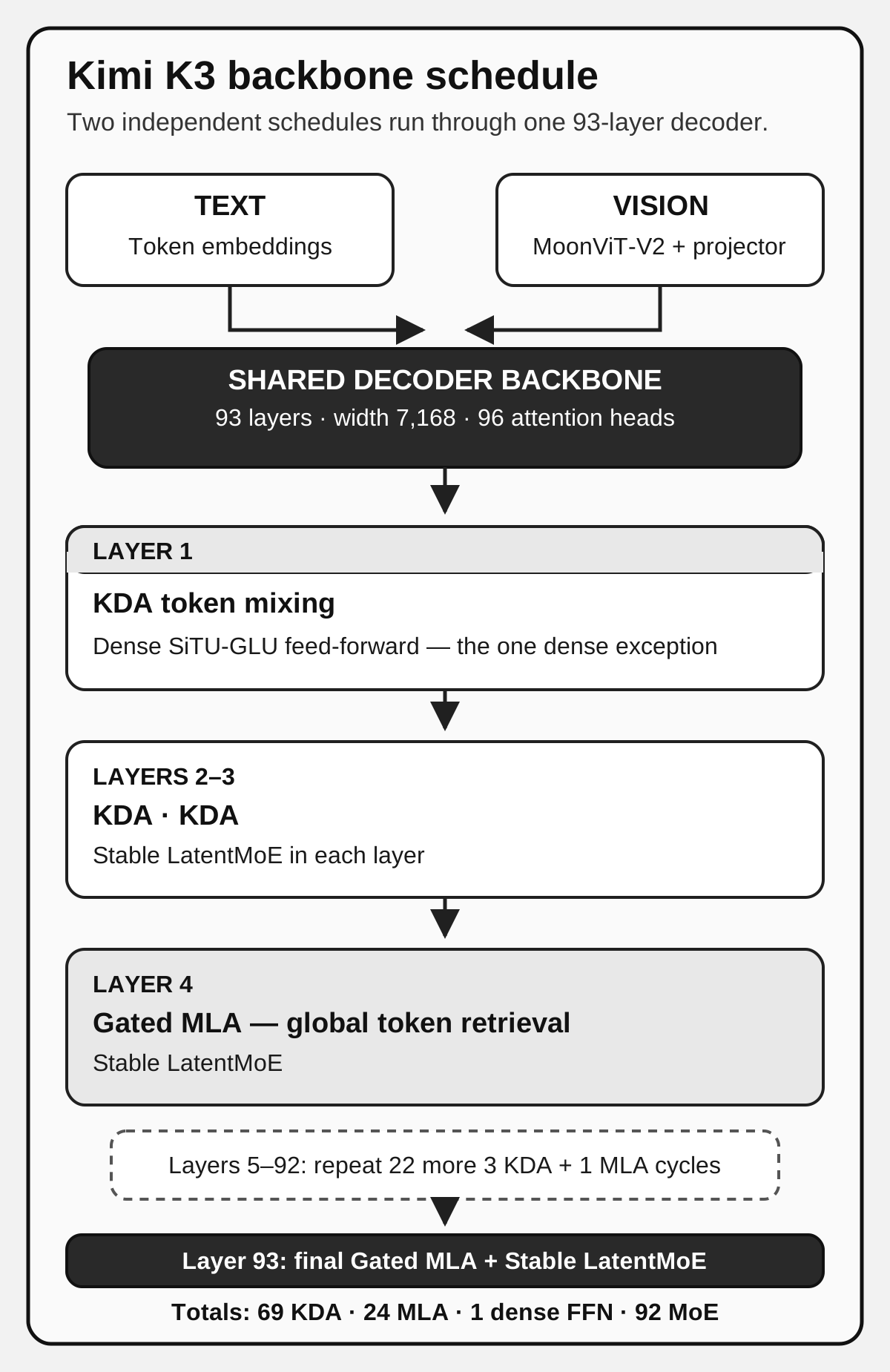
The first decoder layer is the one exception to the sparse feed-forward pattern: it uses a dense SiTU-GLU MLP. The remaining 92 decoder layers use Stable LatentMoE. This diagram is an explanatory synthesis of the released configuration and report, not a literal execution trace.
The two schedules are independent:
The 23 attention macrocycles account for layers 1–92. Layer 93 is the additional MLA, so the backbone ends with global attention. This yields 69 KDA layers and 24 MLA layers. The official configuration lists every attention layer explicitly.
A compact architecture card
| Quantity | Kimi K3 |
|---|---|
| Model type | Native multimodal sparse MoE decoder |
| Total parameters | 2.78T in the report; rounded to 2.8T in the model card |
| Activated parameters | 104.2B per token |
| Backbone layers | 93 |
| Hidden width | 7,168 |
| Attention heads | 96 |
| Attention head width | 128 in KDA; 192 for MLA queries/keys and 128 for MLA values |
| Attention composition | 69 KDA + 24 Gated MLA |
| Routed experts per MoE layer | 896 |
| Routed experts selected per token | 16 |
| Shared experts | 2 |
| Routed latent width | 3,584 |
| Hidden width inside each routed expert | 3,072 |
| Dense feed-forward layers | 1; subsequent layers use MoE |
| Vocabulary | 163,840 entries in the released config, reported as 160K |
| Maximum context | 1,048,576 tokens |
| Vision encoder | MoonViT-V2, 401M parameters, 27 layers, 12 heads, patch size 14 |
| Post-training expert quantization | MXFP4 weights, MXFP8 input activations |
These are architecture and release facts from the K3 technical report, official repository, and released model configuration at revision 9f62e4e. They do not tell us how capable the model is. They tell us what kind of computation it performs.
Four distinct meanings of “memory”
K3 discussions become confusing when one word is used for four objects:
| Memory | Lives where? | Persists for how long? |
|---|---|---|
| Learned knowledge | Model parameters | Across requests until weights change |
| KDA recurrent state | One fixed matrix per KDA head and request | Across tokens in the active sequence |
| MLA KV cache | In the report’s production design, a compressed 576-value payload per token and MLA layer under the released factorization | Across decode steps for the active sequence |
| AttnRes block representations | Earlier computational depths | Recomputed within one model forward call; not stored in the autoregressive cache |
None of these is a user-facing memory database. None automatically persists from one unrelated API request to another. The K3 serving system can cache shared prefixes, but that is reuse of model state for an identical token prefix, not autobiographical memory.
1. The GPT-2 baseline: preserve every token separately
GPT-2 is a useful starting point because its decoder block is clean. GPT-2 small has 12 layers, hidden width 768, and 12 attention heads. Depending on counting conventions it is often described as roughly 117M or 124M parameters. We will use the common 124M count only when reproducing the “how many GPT-2s?” size analogy; the original architecture and training account is OpenAI’s GPT-2 report.
For a batch of token IDs, let:
where is batch size, is sequence length, and is model width. In one attention head, learned projections produce:
For one batch item, causal softmax attention is:
is zero on positions the token may read and negative infinity in the future. Each query row competes over all eligible key rows. That gives standard attention its defining strength: every earlier token remains separately addressable.
A shape walkthrough
Take a toy prompt with four tokens, one head, and head width three:
Q: [4, 3]
K: [4, 3]
V: [4, 3]

Q @ K.T -> scores:  [4, 4]
softmax(scores) ->  [4, 4]
weights @ V ->      [4, 3]
Row 4 of the score matrix answers: “For token 4’s query, how relevant is each of tokens 1 through 4?” At training or prefill time, the model computes a row for every position. At decode time, the new token contributes one query, one key, and one value; its query compares with all cached prior keys.
Why precise retrieval is valuable
Suppose the context contains:
The access code for the west door is 1847. … 80,000 tokens later … What is the west-door code?
A full-attention head can make the final query assign a high score to the earlier token span around 1847. The representation is distributed, and there is no guarantee that a particular head performs this lookup, but the architecture preserves the option. Token 37,412 has not been blended irreversibly into a single summary.
Prefill and decode are different workloads
During prefill, the prompt’s tokens are processed together. Exact full attention evaluates all permitted query-key pairs. Its arithmetic is quadratic in sequence length: .
During decode, one new token is generated at a time. Old keys and values do not change, so each full-attention layer stores them in a KV cache. The next query reads a cache whose length grows with the context. Per-token attention work and cache traffic therefore grow with prior sequence length.
prefill:  N queries x N keys, computed in parallel
decode:   1 new query x N cached keys, repeated token by token
This distinction will matter repeatedly. A method may accelerate prefill but not decode, or may replace the decode cache while making prompt processing harder to parallelize.
What FlashAttention fixes—and what it does not
The naive implementation writes the score and probability matrices to high-bandwidth memory. FlashAttention tiles exact attention so that smaller pieces remain in fast on-chip memory; it keeps running softmax statistics and avoids materializing the whole score matrix in HBM.
This is a profound systems improvement. It does not change exact full attention into a linear-arithmetic algorithm. The pairwise dot products still exist. A precise statement is:
FlashAttention reduces memory traffic and auxiliary storage for exact attention; it does not remove exact attention’s quadratic pairwise arithmetic during prefill.
The first bottleneck
At one million tokens, retaining individually addressable entries is powerful and expensive. The prompt must pay pairwise attention in every global-attention layer, and decode must repeatedly move cached information.
So the first architectural question is:
Can we replace the growing list of prior keys and values with a fixed-size sufficient state?
2. Linear attention: compress the history into a matrix
Ignore softmax for a moment and consider:
Matrix multiplication is associative:
The two parenthesizations construct different intermediate objects:
- has shape and grows with the sequence.
- has shape and depends on feature widths, not .
That second object suggests a recurrent state. Using a feature map on queries and keys, maintain:
Then read:
is fixed in shape. supplies normalization. Causal processing follows naturally because the state at includes only tokens up through .
This feature-map formulation is the important qualification. Softmax is applied to query-key pair scores and cannot simply be moved through the multiplication. Transformers are RNNs uses kernel feature maps to make the query-key similarity separable and thereby exposes the linear recurrent form.
Misconception: Linear attention is not ordinary softmax attention with faster parentheses. Changing the kernel or recurrence changes the function class.
The associative-memory interpretation
An outer product updates a matrix so that a later query aligned with retrieves components of :
That makes look like associative memory: keys act as learned address directions and values as learned payloads. Linear Transformers Are Secretly Fast Weight Programmers makes the relationship explicit. A slow network, whose parameters are learned by backpropagation, emits keys and values that program a fast-changing matrix during the forward pass.
The word fast refers to time scale, not wall-clock speed:
- ordinary model weights change across optimizer steps;
- the fast-weight matrix changes at every token.
A two-dimensional memory
Let:
After one additive write:
Read with the same direction:
Now write an overlapping key:
The state becomes:
Reading the first key now returns:
The second association leaked into the first. The keys overlap, so their outer products interfere.
Real heads have learned, normalized, high-dimensional keys. Multiple heads can distribute associations. Yet the capacity fact remains: a fixed-size matrix cannot preserve an unlimited number of arbitrary bindings without collision.
What was gained and lost
| Property | Full attention | Additive linear attention |
|---|---|---|
| State across decode | Grows per token | Fixed matrix |
| Individual token remains addressable | Yes | No; history is compressed |
| Sharp competition over all tokens | Softmax provides it | Only approximated or replaced |
| New association | Append a new KV entry | Add an outer product |
| Delete or replace | Old token remains separately stored | No native delete in pure additive state |
This exposes the next problem:
If memory has fixed capacity, how should it overwrite old content rather than merely piling on another association?
Notation reset: from normalized features to fast weights
The feature-map equations above are the canonical linear-attention background. Their extra denominator state normalizes the read, making it resemble a normalized attention average. DeltaNet and KDA are usually written in a different, unnormalized fast-weight notation: the state itself learns key-to-value predictions, and the delta update corrects those predictions directly.
From this point onward, and mean the learned query and key vectors used by that fast-weight system. The symbol belongs only to the normalized feature-map construction above. DeltaNet and KDA have no denominator recurrence. Later, will name a newly computed decay-logit vector; it is unrelated to and is not persistent state.
3. DeltaNet: write the error
Pure additive memory writes the requested value whether or not the memory already predicts it. DeltaNet first asks what the current state would return under the new key:
It computes the mismatch:
then writes only that error:
is a learned write strength. Expanding gives:
The first term removes the old prediction along the key direction. The second installs the new target association.
Why this is an online learning step
Consider the instantaneous reconstruction loss:
The gradient with respect to is:
One gradient step with learning rate is exactly the delta update:
This is the deepest conceptual turn in the attention genealogy:
The recurrent state is a tiny linear predictor being trained online inside the forward pass. The surrounding neural network learns what keys, target values, and per-token learning rates make that inner learner useful.
The “fast weights” are not updated by the outer optimizer during inference. The outer optimizer has already learned the rule that generates their updates.
A complete overwrite
Suppose the current state maps:
Now the same key should return:
The current prediction is , so:
With , the correction is:
Adding it changes the relevant state row from to . Reading returns the new value exactly.
That exact-overwrite statement assumes a unit-length key: . More generally, reading the update back through the same key multiplies the correction by , so alone is not enough for an exact replacement. KDA makes this assumption concrete by L2-normalizing its queries and keys before the recurrence.
What the delta rule does not solve
The update is targeted. It changes the state in the direction selected by the current key. That is ideal when one association must be corrected.
It does not answer a broader question such as: “The code file has changed, the earlier implementation details are now stale, and several related features should fade.” Nor does it automatically clear diffuse interference that does not line up with the present key.
So we need two operations:
- surgery: update one addressed association;
- decay: reduce the influence of stale state more broadly.
4. Gated DeltaNet: give memory a lifetime
Gated DeltaNet combines a delta update with a data-dependent retention gate. Using the K3 matrix orientation, a simplified scalar-gated rule is:
where controls how much prior state survives.
The two gates answer different questions:
- : How much existing memory should remain?
- : How forcefully should this key-value correction be written?
If , the old state does not decay globally. If , every component is halved before the targeted update. Repeated retention gives exponential memory:
For constant , the half-life is:
An of 0.99 has a half-life of about 69 tokens; 0.999 has a half-life of about 693 tokens. This isolates only multiplicative retention. In a real run, varies by token and channel, while later delta erases, new writes, and overlap among key directions can either destroy or alter a stored association. The calculation is an intuition for the gate’s time scale, not a prediction of an item’s exact survival.
Why one scalar is too blunt
Imagine a conversation switches from planning a Paris trip to debugging code. Some state should disappear quickly: hotel candidates, dates, and neighborhood comparisons. Other features should persist: the user’s identity, communication style, and the fact that the current answer should be concise.
A scalar gate applies one retention value to the entire state. It can forget quickly or slowly, but not both in different learned subspaces at the same step.
This motivates KDA’s central change:
Give different key channels different retention rates.
5. Kimi Delta Attention: channel-wise forgetting
Kimi Linear introduced Kimi Delta Attention as an extension of Gated DeltaNet. K3 keeps the core recurrence but makes two distinct changes. Its lower-bounded decay parameterization has an explicit numerical and Tensor Core motivation. Its full-rank output gate is a separate architectural and modeling choice about what retrieved information enters the residual stream.
For one head:
K3’s report writes:
Now:
There is one retention value per key channel, not one for the whole matrix. Left-multiplying by scales the rows of the old state independently.
Read the recurrence as four verbs
The equation becomes easier if we read it procedurally:
- Retain: scale each row of old memory by its own .
- Erase: subtract what the retained state predicts along the new key, in proportion to .
- Write: add the new key-value association, also in proportion to .
- Read: apply the current query to the updated state.
The exact multiplication order matters. “Retain, erase, write” is not permission to commute the matrices. It is a verbal map of the published equation.
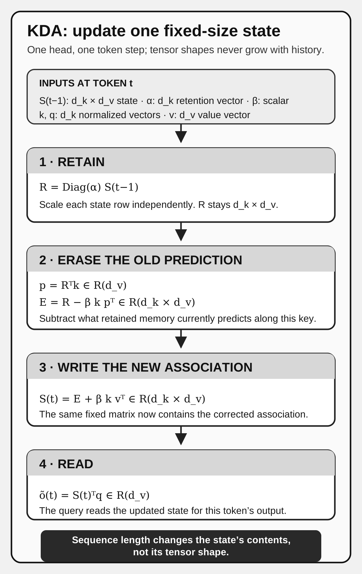
KDA update for one head. The state keeps shape at every token; only its contents change. The diagram follows the published multiplication order rather than treating the four verbs as interchangeable operations.
A channel-wise example
Suppose a two-row state is:
A scalar retention of 0.5 yields:
KDA can instead choose:
giving:
One learned direction survives almost intact while the other nearly clears. The rows are not literally labeled “durable fact” and “temporary topic.” Training is free to discover directions with useful time scales.
Where , , , , and come from
In K3, each token representation is projected into these quantities. The KDA query, key, and value paths use a short convolution followed by Swish; queries and keys are L2-normalized. A low-rank projection plus a head-specific bias produces a channel-wise decay logit. A separate learned projection produces the scalar write strength for each head. The released implementation exposes these pieces in KimiDeltaAttention.
The short convolution has kernel size four in the released configuration. It gives each projection a tiny amount of local token mixing before the long-range recurrence. This is not the main memory; it is a short local preprocessor whose state must also be cached during decoding.
A third gate: control what leaves the module
After the recurrent read, K3 replaces Kimi Linear’s low-rank output gate with head-wise RMSNorm and a full-rank, input-dependent output gate:
We now have three separate controls:
- controls survival of old memory;
- controls the current correction strength;
- controls which retrieved channels enter the residual pathway.
This distinction is easy to miss. A memory may retain information without exposing all of it on every token.
The report presents this full-rank output gate as a modeling change. Unlike the lower-bounded decay below, it is not justified as a requirement for the 16-token Tensor Core tiling argument.
K3’s lower-bounded decay
Chunkwise KDA needs cumulative products of retention values. If a per-step retention can become arbitrarily close to zero, reciprocal cumulative factors can overflow in finite precision.
Kimi Linear used an unbounded negative-Softplus log-decay. Let
denote the newly computed, channel-wise decay-logit vector for token in one head. It is produced from the current token representation; it is not recurrent state and is unrelated to the normalized-linear-attention denominator introduced in Chapter 2. K3 maps it to:
Therefore:
The lower limit is , but the one-step retention is strictly greater than that value because a sigmoid never reaches its endpoint. In mathematical language, is the infimum, not an attained minimum. That may sound like a memory-quality choice, but the report emphasizes a systems consequence. Over a 16-token tile, cumulative log-decay stays above , so the reciprocal stays below and within BF16’s dynamic range. Both diagonal and off-diagonal causal tiles can then use dense Tensor Core matrix multiplication instead of a slower explicit position-pair path.
Evidence: The bound, , 16-token tile argument, and Tensor Core consequence are from K3 report §2.1.1.
Interpretation: This is a textbook example of architecture and kernel design becoming one decision. The gate is constrained not only because of modeling preference but because a bounded numerical range unlocks a better implementation.
What “fixed-size” means at K3 scale
The released K3 KDA shape is 96 heads, with . One layer’s recurrent state contains:
numbers per request. In BF16 that is about 3 MiB. Across 69 KDA layers:
numbers, or roughly 207 MiB in BF16.
This is a derived estimate from the released dimensions. It excludes short-convolution state, padding, metadata, alignment, snapshots, and any higher-precision or sharded representation used by a particular engine.
The lesson is important:
Constant in sequence length does not mean small in absolute terms. KDA replaces growth with context by a substantial but bounded per-request state.
What KDA is not
KDA is not a collection of one slot per old token. It cannot point back to arbitrary token 37,412 after that token has been compressed into the state. It is not ordinary softmax attention under another kernel. It is a learned recurrent memory whose update rule retains the query-key-value vocabulary of learned addressing.
That fixed capacity forces the hybrid design we will reach in Chapter 7.
6. The GPU problem: a recurrent idea on a parallel machine
The simple KDA recurrence has a serial dependency:
GPUs prefer large, regular matrix multiplications with many operations in flight. A recurrence may use fewer theoretical FLOPs than full attention and still lose wall-clock time if it launches a long chain of tiny kernels.
Chunkwise execution
KDA divides a sequence into chunks:
tokens:  [ chunk 1 ][ chunk 2 ][ chunk 3 ] ... [ chunk m ]
state:       S0  ----> S1  ----> S2  ---->           Sm
Figure 2. KDA remains recurrent across chunks while algebra exposes parallel work within each chunk.
For a chunk of tokens:
- the incoming state summarizes preceding chunks;
- causal interactions among the local positions are computed with dense matrix operations;
- the outgoing state is passed to the next chunk.
Linear-attention implementations commonly experiment with chunks such as 64 or 128 tokens, but chunk size is a hardware and workload tuning parameter, not a property of the recurrence. Smaller chunks expose less parallel work; larger chunks do more local pairwise work and consume more temporary storage.
K3’s report describes a UT transform and a pseudo-value term that permit this split. The delta-rule literature relates the rank-one state transitions to generalized Householder transformations, while Kimi Linear exploits a specialized diagonal-plus-low-rank structure. You do not need to reproduce the full derivation to retain the key fact: the recurrence’s meaning is sequential, while its implementation batches much of the local work.
The local causal matrix keeps its diagonal because token reads the state after token has updated it. That remains causal for next-token prediction: the representation at may use the observed token at while predicting token .
The lower-bounded decay from Chapter 5 matters here because cumulative-decay rescaling remains numerically bounded inside 16-token tiles.
Training, prefill, and decode use different paths
The official implementation makes the regimes visible:
mode = "fused_recurrent" if use_cache and q_len == 1 else "chunk"In words:
- training and multi-token prefill: use a chunkwise KDA kernel;
- single-token cached decode: use a fused recurrent kernel.
The released code delegates these to chunk_kda and fused_recurrent_kda in Flash Linear Attention. The report’s production system goes further with FlashKDA, a CUTLASS implementation that overlaps token-parallel work with head-parallel state propagation.
Context parallelism is not simple summation
For additive linear attention, each device can process a segment from zero state and preceding devices can sum their contributions. KDA is harder because each token applies a transition matrix to the incoming state:
where:
A segment therefore defines an affine transformation:
Two such segments compose associatively:
This algebra is the basis of KDA Context Parallelism. Each rank computes its local transition and zero-state contribution, exchanges fixed-size fragments, and uses a prefix scan to recover the correct incoming state. Unlike full-attention context parallelism, the communicated state does not grow with segment length.
This gives us a general engineering lesson:
An associative summary is a parallelization primitive. Finding the right composable object can matter as much as reducing FLOPs.
Checkpoint 1
Try these before continuing.
- Why is the KDA state constant in sequence length but not necessarily cheap?
- What is the difference between and ?
- Why can’t KDA Context Parallelism merely sum each rank’s zero-state result?
- Which execution path handles a single cached decode token in the released implementation?
Answers appear in the checkpoint key near the end.
7. Why K3 keeps global attention: MLA as the archive
No matter how good its eviction policy becomes, a fixed-size state cannot preserve arbitrary detail from an unbounded sequence. Better recurrence design moves the quality-efficiency frontier. It does not repeal the capacity limit.
The Kimi Linear work found that a hybrid architecture performed better than treating KDA as a universal replacement. K3 repeats:
KDA -> KDA -> KDA -> Gated MLA
KDA -> KDA -> KDA -> Gated MLA
...
KDA -> KDA -> KDA -> Gated MLA
                               -> final Gated MLA
The final extra MLA ensures the backbone ends with global token-to-token retrieval.
What Multi-head Latent Attention compresses
Ordinary attention caches head-specific keys and values for every token. Multi-head Latent Attention, introduced in DeepSeek-V2, projects each token through a smaller latent bottleneck. The original MLA paper explains how projection absorption can move the key/value up-projections into adjacent query/output projections, allowing inference to keep the compressed latent payload rather than materializing and caching every head-specific key and value. In a simplified content-only view:
then learned up-projections reconstruct head-specific content keys and values used by softmax attention.
This produces a completely different kind of compression from KDA:
- KDA compresses across tokens: the entire prefix becomes one state per head.
- MLA compresses within each token: the K3 report says the production cache keeps a compressed per-token entry; the released factorization makes that payload 512 latent values plus 64 shared-key values, or 576 values per token per MLA layer.
The MLA cache still grows with sequence length. That growth buys token-level addressability.
A useful archive/whiteboard analogy
KDA is a whiteboard. It has fixed area, it can be revised, and important patterns can persist, but enough writing creates interference.
MLA is an archive. Every document retains its own compressed folder. Looking through all folders is more expensive, but a query can recover one specific old item.
K3 uses the whiteboard most of the time and periodically opens the archive.
The analogy should not be pushed too far. MLA does not wait for KDA to “request” a lookup in a symbolic sense; each MLA layer computes learned global attention for every position. The useful point is the division of capacity.
NoPE: order without explicit position embeddings
K3 applies no explicit positional encoding to its MLA queries or keys. There is no RoPE retuning when extending context. KDA’s ordered recurrent updates, short convolutions, gates, and decay make the sequence representation position- and recency-sensitive before MLA performs global content interaction.
This does not make position irrelevant. A recurrence is inherently ordered: processing then generally yields a different state from processing then . “NoPE” means the model does not add a separate explicit positional-encoding mechanism to the attention projections.
The released MLA shapes, without hand-waving
The released configuration at the reviewed revision uses:
- a 1,536-dimensional low-rank query bottleneck;
- a 512-dimensional KV content latent;
- 128 non-positional content dimensions per query/key head;
- a 64-dimensional shared key channel retained under the legacy name
qk_rope_head_dim; - 128 value dimensions per head.
Therefore a final query or key head is 192-dimensional, not 128-dimensional:
In the readable implementation, the query up-projection produces 96 heads and splits each into a 128-dimensional q_pass part and a 64-dimensional q_rot part. Because K3 sets mla_use_nope=true, the latter is not actually rotated; q_rot is a legacy variable name, not evidence that RoPE is active.
The combined KV down-projection emits 576 numbers per token:
The 512-dimensional latent is then expanded into 96 head-specific pairs of a 128-dimensional content key and a 128-dimensional value. The same shared 64-dimensional key channel is broadcast across heads and appended to each content key. The result is 192-dimensional keys and queries, paired with 128-dimensional values.
These settings are implementation evidence, not a general definition of MLA.
Implementation boundary: report design versus reference Python
The K3 report says its production cache uses the compressed per-token representation. Under the released factorization that payload is values per token per MLA layer. Projection absorption—the algebra that makes latent caching possible—is explained in the original MLA paper. The public Hugging Face Python at the reviewed revision instead expands each token into 96 head-specific 192-dimensional keys and 96 head-specific 128-dimensional values, then calls
KimiDynamicCache.update. It therefore stores values per token per MLA layer. The public implementation demonstrates the factorization and attention computation, but does not demonstrate the production latent-cache footprint. Both versions still grow linearly with sequence length; they differ by what each token contributes to the cache.
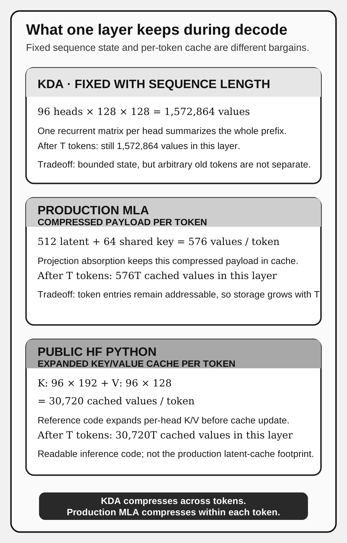
One-layer cache comparison, excluding KDA’s short-convolution state and all implementation overhead. KDA’s recurrent matrix is large but fixed in sequence length; both MLA forms grow per token. The public Python figure is a reference-implementation footprint, not the production serving design.
Gating the global read
K3 also places a full-rank, channel-wise output gate on MLA:
Thus both KDA and MLA can condition which retrieved channels enter the rest of the network. The mechanisms retrieve from different storage, but expose information through a similar learned valve.
During training, K3 keeps the MLA attention output in FP32 to correct a biased rounding error in flash attention. That doubles the on-chip output-tile footprint, so Moonshot redesigned the kernel to overlap the output with KV staging buffers rather than the query tile. It is a small report detail with a large theme: numerical accuracy, shared-memory layout, and pipeline depth are one coupled choice.
The hybrid cost profile
Only 24 of 93 attention layers perform global attention. That reduces, rather than eliminates:
- quadratic prefill arithmetic;
- a per-token-growing cache;
- global cache traffic during decode.
K3 is not a purely linear-time model. It is a deliberately hybrid model that spends exact attention where the authors judged it worth the cost.
8. Stable LatentMoE: scale width conditionally
Attention mixes information across sequence positions. A feed-forward network transforms features within each token position. Mixture-of-Experts changes the latter operation.
In a dense Transformer, every token uses the same feed-forward parameters. In a sparse MoE, a router scores many candidate feed-forward networks and sends each token through only a small subset.
K3 contains 896 routed experts in each MoE layer, selects 16 per token, and also runs two shared experts: 898 conceptual expert modules per MoE layer, though “16 of 896 routed plus two shared” is the accurate description of a token’s path. The routed choice ratio is:
This is what the report calls sparsity 56: one fifty-sixth of the routed expert pool is active for a token. The two shared experts are additional full-width paths, so “1.79% of the whole model runs” would be an incorrect interpretation.
Why total and activated parameters diverge
The full expert pool contributes to K3’s 2.78T total parameters. A single token activates about 104.2B parameters across the model. Total parameters measure the capacity available across possible routes; activated parameters more closely track per-token work.
Activated parameters are still not FLOPs. A matrix’s shape, reuse across a batch, numeric precision, network communication, kernel efficiency, and memory traffic all change wall-clock cost.
LatentMoE’s width bottleneck
Routing through 16 full-width experts would create severe expert-weight and communication traffic. LatentMoE separates the main hidden width from a smaller routed width .
For K3:
A simplified routed path is:
x [7168]
   |
W_down
   v
z [3584] -> router selects 16 of 896 experts
   |          each selected expert: 3584 -> 3072 -> 3584
weighted aggregate u [3584]
   |
RMSNorm -> W_up
   v
routed output [7168]

in parallel: two shared full-width experts process x [7168]
final MoE output = shared paths + routed path
Figure 3. In each MoE layer, Stable LatentMoE keeps ubiquitous transformations at full width and moves conditional specialization into a narrower routed space. The first decoder layer is dense and does not use this routed path.
The report’s equation is:
The released model code follows this shape: routed_expert_down_proj, the selected experts, optional routed_expert_norm, and routed_expert_up_proj, plus shared_experts.
Where almost 2.78 trillion parameters live
The routed expert count lets us sanity-check the scale. Ignoring biases, one gated routed expert has three dominant matrices—gate, up, and down—so its parameter count is:
or about 33.0 million parameters. Across 896 routed experts in one MoE layer:
Across the 92 MoE layers:
That derived estimate already explains nearly all of the reported 2.78T total. The remainder includes the two shared experts per MoE layer, the dense first-layer MLP, embeddings and output head, KDA/MLA projections, latent projections, routers, norms, and the vision system. The precise checkpoint accounting can differ in details, but the order-of-magnitude conclusion is robust: the dormant routed-expert pool dominates total parameters.
A revealing non-choice: K3 does not tie its embeddings
The released configuration sets tie_word_embeddings: false. Its input embedding table and output vocabulary head are separate even though both have shape:
about 1.17B parameters apiece. Together they contribute about 2.35B parameters; tying them would save one table’s roughly 1.17B parameters.
The companion book Inside a Transformer, Slowly explains the powerful inductive bias behind weight tying: by forcing input and output to share coordinates, training encourages compatible token and contextual representations. K3 makes the other legitimate design choice. Untied tables can specialize input lookup and output scoring independently, at the cost of the extra table. The configuration establishes the choice; it does not by itself establish why Moonshot preferred it.
Why “Stable” was necessary
The routed branch chains a down-projection, a gated expert, and an up-projection. At K3 scale the authors observed two failure modes:
- internal activation growth in the routed computation;
- expert-load imbalance severe enough to create stragglers and poorly trained experts.
Stable LatentMoE addresses scale instability in three places.
1. Normalize the expert aggregate
The scale of depends on which experts were selected, their outputs, and their routing weights. RMSNorm before prevents the up-projection from receiving an uncontrolled routed scale. The report says this improved validation loss and downstream results in addition to stabilizing training.
2. Bound the gated activation with SiTU-GLU
SwiGLU multiplies two unbounded factors:
Large coincident coordinates can produce outliers, especially troublesome in low precision. K3’s Sigmoid Tanh Unit GLU applies smooth caps:
K3 uses and . Near zero, , so the response resembles SwiGLU locally. At large magnitude, each branch is bounded, and their product has magnitude at most in the scalar case.
This is not merely “use tanh because it is stable.” It is a designed compromise: preserve the useful local and positive-side behavior of SwiGLU while capping extreme products.
3. Balance routing by targeting a quantile
The router computes sigmoid scores:
An expert-specific bias affects which experts enter the top 16:
But the mixture weights use the original scores, normalized over selected experts:
This separation is subtle and valuable. The bias regulates dispatch without directly changing the mixture’s output weights or the router’s gradient objective.
Older auxiliary-loss-free balancing adjusts biases by fixed steps, which trades slow correction against oscillation. Quantile Balancing estimates the bias each expert would need to receive its target share of the global batch. With tokens, experts, and choices per token, the target load is:
K3 obtains each token’s selection cutoff from Top- scores, computes expert margins relative to those cutoffs, and chooses the corresponding quantile. At scale, it estimates those quantiles from all-reduced histograms instead of gathering millions of margins. The update applies to the next batch, and the final bias is frozen for inference.
The router still learns semantic specialization by gradient descent. Quantile Balancing is a separate control loop that prevents the hardware and training data from collapsing onto a few popular experts.
MoE is not a sequence-memory mechanism
MoE decides which parameters transform this token. KDA and MLA decide what information from other token positions reaches it. A token can be routed to a code expert and still fail to retrieve the relevant function definition; the axes are complementary.
9. Attention Residuals: retrieve across depth
So far we have discussed memory across token positions. A separate information bottleneck appears across layers.
In a pre-norm residual stack, we can schematically write:
Every earlier module output is added with coefficient one. A later layer receives one accumulated vector, not a menu of earlier computational stages.
Residual connections make deep networks trainable, but uniform accumulation has side effects. The Attention Residuals paper reports hidden-state growth and dilution of individual layer contributions with depth.
The conceptual move
Transformers replaced a recurrent sequence bottleneck with attention over earlier positions. AttnRes applies the same selection idea to depth: let a later layer attend over outputs from earlier layers.
For full AttnRes, the token embedding and previous module outputs act as keys and values. Each destination layer has a learned pseudo-query . A simplified score is:
The pseudo-query belongs to the destination layer. The source representations depend on the current token and context, so the resulting weights are content-dependent even though the query vector itself is shared across tokens.
RMSNorm matters because otherwise a large-magnitude old layer could win by scale rather than alignment.
A tiny depth-retrieval example
Suppose a late layer can access four earlier representations and produces scores:
Softmax gives approximately:
The late layer receives mostly the fourth representation, some of the second, and little of the others. A conventional residual sum would assign all four coefficient one before later normalization.
AttnRes does not guarantee that old representations remain semantically pure. It guarantees a selectable path to earlier computational states.
Why block the layers
Full AttnRes must keep all preceding layer outputs alive. With fewer than 100 layers, the depth-attention arithmetic is modest; memory and cross-pipeline communication are the practical problem.
Block AttnRes groups module outputs into sums. K3 uses blocks of 12 layers. Later modules choose among:
- the original embedding source;
- completed earlier block sums;
- the current block’s partial sum.
K3 partitions its 93 layers into eight layer blocks, with the last block partial. Counting the embedding source yields nine possible block-level sources near the end.
embedding -> [layers 1-12] -> [13-24] -> ... -> [85-93]
    |              |             |                 |
    +--------------+-------------+-----------------+
                   selectable block sources
                              |
                         later module
Figure 4. Block AttnRes exchanges per-layer history for a much smaller set of block-level representations while preserving a current partial sum.
The report states that about eight blocks recovered most of full AttnRes’s benefit across model scales. Block-level storage reduces the overhead from to , where is the number of block sources.
The released implementation is pleasantly literal
The official function _apply_attn_res:
- concatenates prior
block_residualvalues with the currentprefix_sum; - RMS-normalizes them to create keys;
- projects them to one score per source;
- softmaxes across sources;
- takes the weighted sum of the unnormalized values.
This code is worth reading because it demystifies the mechanism. AttnRes is not another full attention head over token positions. For each token independently, it performs a tiny attention operation over depth sources.
There is an important lifetime boundary in the released implementation. KimiLinearModel.forward starts with block_residual=None; when AttnRes is enabled, its block-source tensor is built fresh inside that call. KimiDynamicCache preserves KDA’s convolution/recurrent state and MLA’s keys and values, but it does not preserve block_residual.
So AttnRes is depth memory only within the current forward computation. During a multi-token prefill call, each prompt position can select among the depth sources constructed for that position as it passes through the network. During cached single-token decode, the new token gets a fresh depth-source stack across the 93 layers. The next generated token starts another stack. AttnRes is not another store of autoregressive sequence history.
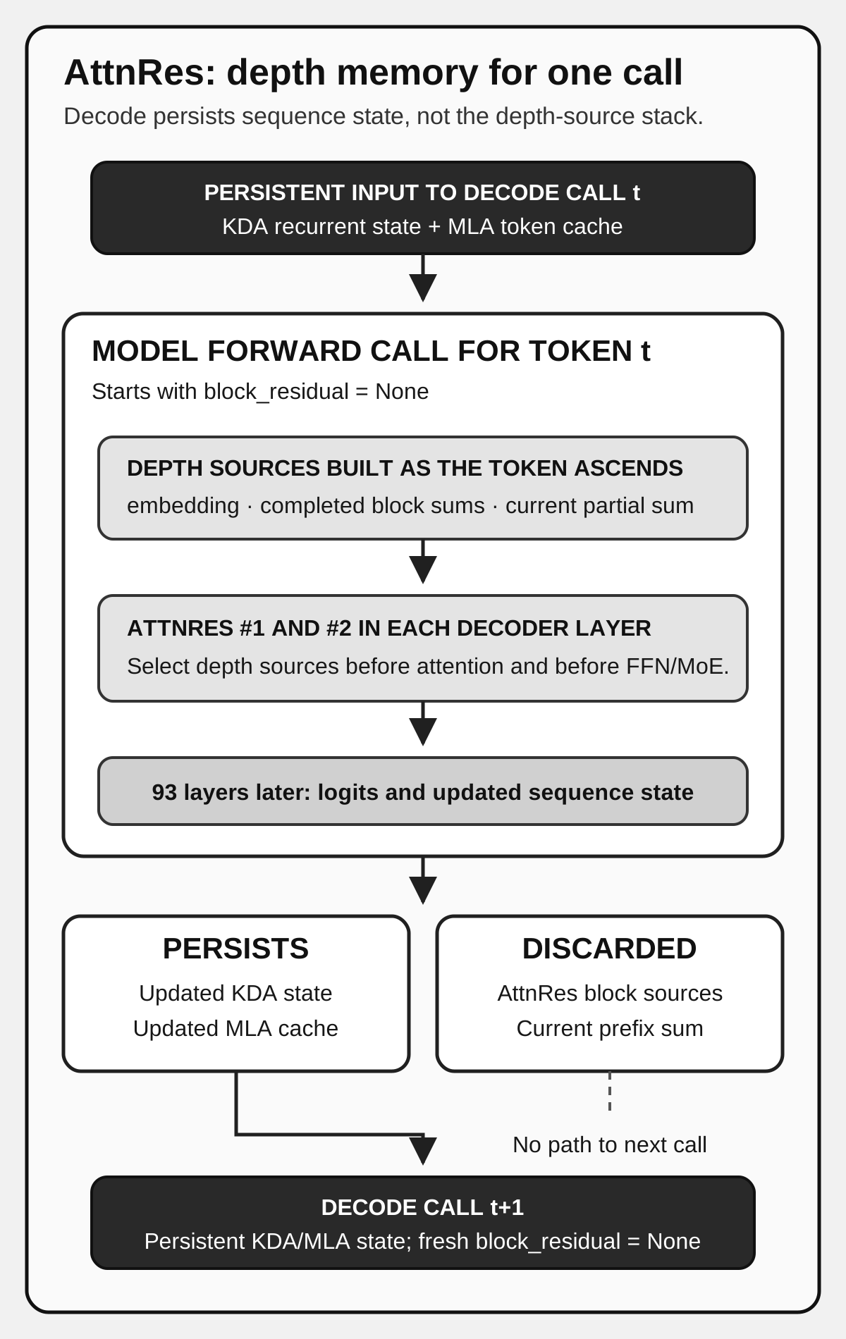
AttnRes lifetime during cached decode. The generated token’s KDA recurrent state and MLA cache survive into the next decode step; its AttnRes depth-source stack does not.
MLA versus AttnRes
| Question | MLA | AttnRes |
|---|---|---|
| What is selected? | Token positions | Earlier computational depths |
| Selection set grows with | Sequence length | Number of block sources |
| Main failure addressed | Lost token-level detail | Diluted intermediate representations |
| Cache/state | Production design: per-token latent KV entries | Current-forward block representations; not autoregressively cached |
Calling both “long-context mechanisms” hides the useful distinction. MLA expands accessible sequence history. AttnRes expands accessible computation history.
10. Assemble one K3 layer and the full backbone
We can now read K3 as a division of labor rather than a list of inventions.
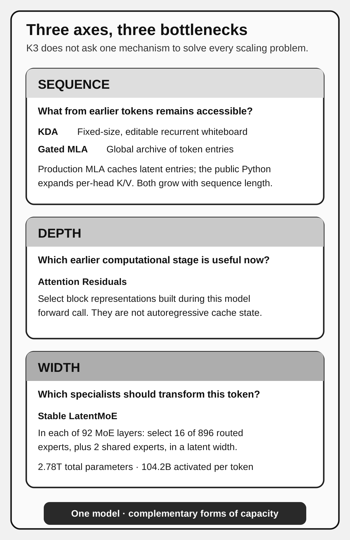
Figure 5. The three principal scaling axes are complementary. AttnRes’s depth sources live only within the current forward call; Stable LatentMoE appears in each of the 92 MoE layers, not in the dense first layer.
Sequence — KDA
- Buys: a fixed-size, editable running state.
- Cannot guarantee: exact recovery of an arbitrary old token after the prefix has been compressed.
Sequence — Gated MLA
- Buys: global softmax retrieval from token-level history, with a 576-value per-token payload under the released production factorization.
- Cannot guarantee: constant memory in sequence length.
Width — Stable LatentMoE
- Buys: enormous conditional channel capacity while activating only a small expert subset for each token.
- Cannot guarantee: retrieval of context that token mixing failed to provide.
Depth — Block AttnRes
- Buys: selective access to earlier computation within the current forward call.
- Cannot guarantee: more persistent token-history capacity across decoding steps.
Modality — MoonViT-V2 plus projector
- Buys: image and video features in the same backbone context as text.
- Cannot guarantee: image generation; K3 has no image-generation decoder.
One decoder layer in conceptual pseudocode
The released code uses a more involved AttnRes prefix-sum schedule, but this pseudocode captures the roles:
def conceptual_k3_layer(x, depth_sources, layer_index):
    # Select useful earlier computational representations.
    x = attention_over_depth(x, depth_sources)

    # Mix information across token positions.
    if layer_index in KDA_LAYERS:
        token_update = kda(rms_norm(x))
    else:
        token_update = gated_mla(rms_norm(x))
    x = update_depth_state(x, token_update)

    # Mix channels, densely in layer 1 and sparsely afterward.
    if layer_index == 1:
        channel_update = situ_glu_mlp(rms_norm(x))
    else:
        channel_update = stable_latent_moe(rms_norm(x))
    x = update_depth_state(x, channel_update)

    return x, depth_sources
This is explanatory pseudocode, not a drop-in implementation. In the actual K3 code, AttnRes is applied separately before attention and before the MLP/MoE, current block outputs accumulate into a prefix sum, and completed block sources are held for the rest of that model-forward call. They are not written into the autoregressive cache.
Follow one token through a macrocycle
Imagine the current token is inside a long code-editing trajectory.
- AttnRes selects a mixture of earlier block representations useful at this computational stage.
- KDA 1 reads and updates its recurrent state, perhaps preserving current task constraints.
- Stable LatentMoE routes the token through 16 specialists in a 3,584-dimensional latent space, plus shared experts.
- KDA 2 and KDA 3 repeat sequence-memory updates at deeper feature transformations.
- MLA compares the token against compressed cache entries for the actual token history, recovering precise evidence that fixed-state KDA may have blurred.
- The next macrocycle receives both evolved token representations and selectable depth sources.
No module is handed a symbolic role. Training jointly learns the representations that make this division useful.
What stayed the same from GPT-2
- causal next-token prediction;
- token embeddings and a decoder backbone;
- attention-like learned retrieval;
- per-token channel transformation;
- normalization and a residual information path;
- logits over a vocabulary.
What changed
- most token mixing is recurrent and fixed-state rather than globally pairwise;
- periodic global attention uses within-token latent compression;
- channel mixing is sparsely routed through a large expert pool;
- depth aggregation is learned rather than uniformly additive;
- visual features are trained into the same backbone from the start;
- low-precision deployment and long-horizon agent behavior influence training itself.
Code-reading map
If you open the official modeling_kimi_linear.py at revision 9f62e4e, follow this order:
KimiDynamicCache— see the two cache families: convolution/recurrent state for KDA and expanded per-head K/V tensors for MLA. Remember that this readable Python cache differs from the report’s production latent-cache design.SituAndMul— the bounded gate and optionally bounded up branch.KimiMLAAttention— query/KV bottlenecks, global attention, and output gate.KimiDeltaAttention— projections, short convolution, decay/write signals, chunk versus recurrent kernels.KimiMoEGateandKimiSparseMoeBlock— top-k routing, latent projections, selected experts, shared path._apply_attn_res— attention over depth sources in about a dozen substantive lines.KimiDecoderLayer— how those modules replace the familiar attention-plus-MLP block.KimiLinearModel.forward— layer-specific masks and state threaded through all 93 layers.
The public Python is an understandable, inference-oriented reference implementation. In particular, KimiSparseMoeBlock.forward rejects training mode with NotImplementedError. It is excellent for reading architecture and following inference data flow, but it is not a reproducible K3 training stack. Production training and serving rely on specialized distributed kernels and systems described in the report; reading Python alone will not reveal their behavior or performance.
What it means to inspect or run K3
The official Hugging Face release was about 1.56 TB when this edition was checked. You can inspect its configuration and Python without downloading the weight shards, but self-hosting the full checkpoint is a datacenter-scale exercise, not a sensible Mac experiment. Moonshot lists vLLM, SGLang, and TokenSpeed as supported serving engines and also exposes an API.
The API model always uses thinking and offers low, high, and max reasoning-effort settings. It was trained with preserved thinking history: for multi-turn and tool interactions, the official usage guidance says to pass the prior assistant message back intact, including the returned reasoning_content and tool_calls. Dropping returned reasoning_content while keeping only visible content changes the context the model was trained to continue. That behavior is an interface contract, not a general requirement of every reasoning model.
Checkpoint 2
- Why does MLA’s cache grow even though it is “latent” attention?
- What does LatentMoE compress: sequence history or routed channel width?
- Why can AttnRes weights vary by token even though each destination layer owns one pseudo-query?
- Why is the final layer MLA rather than KDA?
11. Native multimodality: train vision into the same objective
K3 is not merely the text backbone described above. It accepts images and videos through MoonViT-V2, maps their features through a lightweight projector to the language model’s 7,168-dimensional space, and processes those visual tokens in the shared decoder context.
What “native” means in this report
Many multimodal systems begin with a pretrained language model and a separately contrastively pretrained vision encoder, then align the two afterward. K3’s report describes a different recipe:
- initialize MoonViT-V2 from scratch;
- jointly optimize language and vision from the start of pre-training;
- use the same next-token-prediction objective;
- interleave visual and textual tokens in one context.
The authors report that attaching their SigLIP-initialized MoonViT-3D baseline produced persistently higher vision-tower gradient norms and spikes, whereas from-scratch MoonViT-V2 trained more stably and matched that baseline on their vision evaluations.
Evidence boundary: That is Moonshot’s ablation result for this training regime. It does not prove contrastive pretraining is generally useless. At smaller scales or with different data, it may remain valuable.
Why next-token prediction can supervise vision
The model receives visual features followed or surrounded by text that describes, reasons about, locates, edits, or acts on the visual content. To predict those text tokens, gradients flow through the language backbone, projector, and vision encoder.
This encourages visual representations that support language-conditioned tasks: OCR, spatial references, chart reasoning, screenshot inspection, and code-to-render comparisons. A contrastive objective often emphasizes global alignment between an image and its caption; next-token prediction can reward fine-grained details needed to produce a continuation.
This does not mean raw pixels use the text tokenizer. MoonViT-V2 converts pixels into visual feature tokens first.
The vision path in shapes
The released configuration gives MoonViT-V2:
- 27 Transformer layers;
- hidden width 1,024;
- 12 attention heads;
- patch size 14;
- an MLP projector to text width 7,168.
Before projection, a 2-by-2 pixel-shuffle merge reduces visual token count by a factor of four. Images and videos share encoder parameters. Video processing factorizes spatial attention within frames and temporal attention across frames, then uses temporal pooling to reduce the sequence.
The report states support for images up to pixels in this path. At a naive patch size of 14, that resolution would create patch positions before merging. A fourfold token reduction brings the rough spatial count to 16,384, ignoring special tokens and implementation details. This derived calculation shows why token compression matters even inside a one-million-token context.
Data is part of the architecture
K3’s vision corpus includes:
- captions and interleaved image-text documents;
- OCR and perception examples;
- videos;
- visual coding data;
- absolute and normalized coordinate supervision;
- code paired with rendered SVG, 3D assets, web pages, games, and CAD schematics.
Programmatic pairs are especially interesting. Code supplies an exact generative description; the render supplies the visual result. A model can learn relationships among implementation, appearance, and iterative correction.
Vision-in-the-loop agents
The report’s post-training environments let the model write code, inspect resulting screenshots or frames, crop or transform images with tools, and revise the artifact. This is more than single-turn visual question answering. The visual observation becomes another event in a long tool-use trajectory.
What K3’s multimodality does not imply
K3 is a multimodal understanding and agentic model. The report does not describe a diffusion decoder or an autoregressive image-token generator that emits new pixels directly. It can create visual artifacts through code and tools, and reason over images/video; that is different from being a standalone text-to-image foundation model.
12. Pre-training: data, scale, and learning a million-token regime
Architecture determines what the model can represent efficiently. Data and optimization determine which behaviors it actually learns.
The pre-training mixture
The report groups text into four primary domains:
- web text;
- code;
- mathematics;
- knowledge.
Pipelines combine heuristic filtering, classifier quality scores, deduplication, and domain-specific sampling rates selected through smaller-model ablations. Knowledge and mathematics data are also rephrased with varied styles and perspectives, generated chunkwise and checked for fidelity to source documents.
The vision corpus adds the categories from Chapter 11. The exact datasets, token counts, mixture weights, and training compute are not fully disclosed in the report. A reader should not infer them from the architecture table.
Scaling-law search is configuration search
Moving from K2 to K3 changed attention, depth mixing, MoE structure, activation function, context length, and multimodal recipe. Hyperparameters optimal for K2 need not transfer. Moonshot reports retuning:
- batch size;
- peak learning rate;
- tokens per parameter;
- model shape;
- learning-rate schedule.
Their fitted held-out curves attribute an approximately 2.5-fold scaling-efficiency gain over K2 to the combined architecture, data, and training recipe. Because several variables changed together, the headline is a system-level result, not a clean causal estimate for KDA alone.
The report says cosine decay beat Warmup-Stable-Decay after each schedule received its own hyperparameter search. This qualification matters. Comparing two schedules with one shared peak learning rate and batch size can accidentally compare “well tuned” against “poorly tuned.”
K3 uses a 1% linear warmup, cosine learning-rate decay, weight decay 0.1, and the weight-clipping mechanism introduced for Kimi K2. Matrix parameters use Muon; attention projection momentum matrices are orthogonalized per head rather than as one full coupled matrix. The stated intuition is that this prevents high-scale heads from dominating the normalization of smaller-scale heads.
Progressive context extension
Training every token at one-million length from the beginning would be extraordinarily expensive. K3 uses a curriculum:
pre-training:       8K  -> 64K
cooldown phases:  256K -> 1M
Only a small fraction of the overall budget pays the longest-sequence cost. The model gradually adapts to larger ranges.
Because K3 uses NoPE, it does not need to rescale RoPE frequencies or interpolate a learned absolute-position table. That removes one context-extension issue, not all context-learning issues.
Length is not dependency
A million-token sequence does not automatically teach million-token retrieval. Natural long documents can contain duplicates, binary debris, truncation, invalid logs, low-quality video segments, and long stretches irrelevant to any target.
The K3 pipeline therefore:
- applies exact and fuzzy deduplication;
- uses perceptual frame hashing for video;
- filters by heuristics and classifiers;
- validates structure;
- upsamples genuinely long coherent sources;
- synthesizes sequences in which tasks require information scattered across the full context.
That last item is crucial. Context length describes how many tokens fit. Long-range capability requires gradients that reward using far-away information.
A practitioner’s reading of the recipe
Four principles generalize beyond K3:
- Retune after architecture changes. Optimizer settings are properties of a model-and-data system, not universal constants.
- Use a length curriculum. Spend most compute where training is economical, then adapt at long lengths.
- Measure dependency, not padding. A long batch is useless if targets can be solved locally.
- Clean long data differently. The failure modes of repositories, videos, and multi-document contexts are not those of short web paragraphs.
13. Post-training: from next-token model to long-horizon agent
K3’s post-training has three main stages:
supervised fine-tuning
        |
        v
reinforcement learning -> 3 domains x 3 effort levels = 9 expert policies
        |
        v
multi-teacher on-policy distillation -> one unified deployed policy
Figure 6. Specialized RL policies explore different domains and reasoning budgets; distillation consolidates them into one model.
Stage 1: supervised fine-tuning as a cold start
SFT establishes tool calling, reasoning format, and baseline agent behavior before RL. Moonshot says it synthesizes trajectories with earlier domain-specialized Kimi models, applies multi-stage verification and human annotation, and serializes interactions with an extensible token markup format.
This is not merely a collection of question-answer pairs. Agent data includes tool calls, observations, reasoning, and actions across long trajectories.
K3 also begins quantization-aware training at SFT, rather than quantizing only after behavior training is finished. We will return to that decision.
Stage 2: nine RL experts
RL is split across three domains:
- general tasks: knowledge, reasoning, vision, faithfulness, search, and professional work;
- general agents: long-horizon assistance, deep research, and paragraph-level writing;
- coding agents: software engineering, coding experience, GPU kernels, and web development.
Each domain trains low-, high-, and max-effort policies, producing nine specialized teachers.
Reasoning effort is trained with a per-problem budget. If an initial policy suggests budget for problem , a trajectory exceeding receives reward . For general tasks the budget counts thinking tokens; for agentic work it counts cumulative output, including reasoning and tool-call arguments. Training starts with a larger and anneals it to obtain lower-effort policies.
This turns “reasoning effort” into a learned conditional behavior, not merely a decode-time max_tokens setting.
Partial rollouts: do not wait for the longest agent
Long-horizon trajectories have severe tail latency. Some agents finish in a few calls; others run for hundreds or thousands. A synchronous RL batch that waits for every rollout wastes hardware.
K3 pauses generation when a fraction of the active trajectories completes, optimizes on completed prompt groups, and queues unfinished rollouts for later iterations. That increases utilization but makes resumed trajectories off-policy: the model may have changed since their earlier tokens were generated. The report says per-token regularization constrains policy updates locally enough to tolerate this staleness.
This is a systems-algorithm trade: accept controlled off-policy data to avoid waiting for stragglers.
Rewards for work without a simple checker
Code tests and exact-answer problems can provide verifiable rewards. Writing and professional tasks often cannot. K3 uses an agentic generative reward model that:
- reads the output;
- creates a rubric;
- scores each candidate against it;
- records scores in a scorepad.
To discourage verbose reward hacking, candidates that exceed a problem-specific length budget automatically lose the binary comparison.
This does not make subjective reward objective. It makes the judging process more structured and constrains one obvious exploit.
Stage 3: Multi-Teacher On-Policy Distillation
A user does not want to load nine separate K3 policies. Multi-Teacher On-Policy Distillation selects the teacher matching the sampled domain and effort, then supplies a dense token-level signal comparing teacher and student probabilities.
The report defines a clipped log-ratio reward:
The student samples its own on-policy trajectories, while the appropriate teacher evaluates those sampled tokens. Clipping limits extreme signals. This consolidates domain and effort behavior without simply concatenating nine offline datasets.
Training the environments, not just the policy
K3’s report is unusually concrete about task generation:
- a configurable white-box environment varies tool interfaces, system prompts, memory, skills, subagents, and context management rather than overfitting one harness;
- a recursively expanded knowledge graph guides retrieval of specialized source material and task synthesis;
- verifiable search, professional, visual, software, kernel, personal-assistant, web-development, and autonomous-execution tasks provide long-horizon experience;
- mock Gmail, Notion, Slack, and Canvas-like applications create reproducible persistent workflows without external API limits;
- visual agents can crop, zoom, transform, calculate, and inspect generated images inside a sandbox;
- kernel rewards combine correctness thresholds, performance relative to an expert baseline and roofline, and anti-hacking checks.
The general lesson is that agentic RL depends as much on environment engineering and verification as on the policy-gradient formula.
Deployment-aware post-training
The 2.78T parameter pool makes deployment memory a first-order constraint. K3 quantizes MoE expert weights—the dominant parameter storage—to MXFP4 and uses MXFP8 expert input activations. Attention, latent projections, shared experts, and routers remain at higher precision.
Quantization-aware training runs through SFT and RL. Rollout and training use the same numeric scheme, avoiding a policy trained in one precision and sampled in another.
K3 also pretrained one multi-token-prediction layer and later fine-tuned it into an EAGLE-3-style draft model for speculative decoding. The target model is frozen; the draft learns from low-, mid-, and high-level AttnRes block outputs and is unrolled for seven steps during training. Instead of only minimizing KL divergence, the report directly optimizes the negative log of the draft-target acceptance overlap:
That objective matches the serving goal: maximize how often target verification accepts draft tokens without changing the target distribution.
14. Systems co-design: why the equations are only half the model
At K3 scale, a mathematically elegant layer is unusable unless it can be trained, communicated, cached, and scheduled. The report treats infrastructure as a first-class contribution.
Parallelism has several axes
K3 pre-training combines:
- pipeline parallelism with virtual stages;
- expert parallelism;
- ZeRO-1 data parallelism;
- pipeline ZeRO-2 gradient sharding;
- context parallelism.
Each partitions a different object: layers, experts, optimizer/gradient state, or sequence segments. Combining them creates opportunities for overlap and many opportunities for stalls.
Perfect expert balance with MoonEP
Even when Quantile Balancing improves semantic dispatch, a microbatch can send uneven token counts to expert devices. One overloaded rank delays the whole step; variable shapes fragment memory and force host-device synchronization.
MoonEP dynamically creates redundant copies of hot experts so every rank receives exactly the same total routed-token load. The report claims a feasible balance can always be formed with at most redundant experts per rank for experts and expert-parallel ranks. Planning happens online from the current router output; redundant weights are prefetched, and their gradients are reduced back to the home expert.
Perfect aggregate balance produces static computation shapes. That eliminates per-layer host synchronization and enables zero-copy communication into expert-grouped buffer positions.
This is different from Quantile Balancing:
- QB adjusts learned routing bias across training batches so experts receive healthy long-run load.
- MoonEP executes a particular microbatch evenly across hardware, including by temporarily replicating hot experts.
Fit the training state, then hide its movement
K3 uses a unified activation manager whose per-tensor policies include recomputation, FP8 quantization, CPU offload, and remote offload. Activation prefetch overlaps with computation. Other techniques include:
- recomputing MoE dispatch rather than saving large routed intermediates;
- checkpointing AttnRes while keeping completed block sources resident;
- remotely offloading activations to less-loaded pipeline ranks;
- sharding and CPU-offloading gradients;
- gathering only locally owned Muon parameter shards through peer-to-peer transfers rather than materializing every full matrix on every rank.
The recurring strategy is not “never move data.” It is “move or recompute data when another operation can hide the cost.”
Hide vision work in pipeline bubbles
Large images and videos vary greatly in encoder cost. K3 partitions large visual samples across context-parallel devices and divides groups to balance multiple images. It schedules much of the vision encoder’s forward and backward computation into otherwise idle pipeline bubbles, reducing its effective critical-path cost.
Million-token RL needs resumable world state
Agentic trajectories combine two large states:
- the model-side prefix state and caches;
- the environment-side filesystem, processes, tools, and application state.
K3 writes evicted idle prefixes to a CPU external cache pool and later prefetches them. KDA recurrent state and MLA cache blocks move together. An auto-throttling scheduler reduces rollout concurrency as KV pressure rises.
For environments, the report describes AgentENV microVMs with pause/resume, fork, and snapshot. Incremental checkpointing stores dirtied memory pages. Moonshot reports creating 51,219,741 sandboxes across 1,505,678 images during training and evaluation, with observed checkpoint/resume latencies as low as 133/49 ms and memory overcommit up to 6.5 times in its workloads. These are vendor-reported system measurements, not general guarantees for Firecracker or other installations.
Serving a hybrid cache
KDA and MLA have different cache geometries:
- KDA: one large fixed recurrent state per KDA layer and request;
- MLA: per-token cache entries whose count grows with the prefix.
A prefix can be reused only if both states correspond to the same token boundary. K3 packs both page types into one allocation pool and separates physical storage blocks from finer 512-token hash boundaries. Sparse KDA snapshots are stored only at candidate hash endpoints, often conversation-turn boundaries.
On a hit, the engine finds the longest boundary for which MLA blocks and every KDA cache group agree, restores the KDA snapshot into private mutable state, copy-on-writes the partial MLA block, and resumes prefill. Cached KDA snapshots are read-only because mutating shared recurrent state would corrupt every request using that prefix.
This is a subtle consequence of recurrence: a KV-cache page contains immutable old entries, but a KDA state is an evolving summary. Reuse requires snapshots, not shared mutation.
Speculative decoding cannot naively roll KDA back
Suppose a draft model proposes seven tokens. The target processes them, which advances every KDA state. If only the first four are accepted, the state must correspond to four tokens—not seven.
Saving a full KDA matrix after every draft token would multiply large state traffic. K3 instead caches the much smaller projected draft inputs and replays accepted updates on chip. The recurrent loop, short convolution, gates, normalizations, and next draft window are fused.
Again, the state equation shapes the serving design.
Fleet scheduling at one-million context
The report gives a representative coding request with a reusable 400K-token prefix and only 4K new prefill tokens. A cache miss can therefore cost orders of magnitude more than a hit.
K3 uses:
- cache-aware affinity: route the session to the cluster holding its prefix, with a consistently hashed secondary cluster for failure handling;
- budget-based admission control: allocate separate capacity to short and ultra-long request classes so a burst of million-token work cannot starve ordinary requests.
Counting requests is not enough when request cost spans roughly three orders of magnitude. Scheduling must account for tokens, cache locality, and expected compute.
The larger lesson
Model architecture, numerical precision, kernels, distributed execution, RL scheduling, sandbox lifecycle, and fleet policy are coupled. “KDA is ” is not a deployment plan. K3’s design is noteworthy partly because its report follows the recurrence all the way down to prefix snapshots and rollback.
Checkpoint 3
- Why does a reusable hybrid prefix need both an MLA cache match and KDA snapshots at the same token boundary?
- Why start quantization-aware training during SFT instead of quantizing only after RL?
- What are the two different jobs of Quantile Balancing and MoonEP?
- Why does the RL pipeline produce nine teachers and then distill them into one student?
15. A guided reading of the K3 report
The 47-page report is dense but well organized once you know what to ask of each section.
First pass: establish the map
Read the introduction and Figure 2, then stop. Your goal is to locate four flows:
- token mixing: KDA and MLA;
- channel mixing: Stable LatentMoE;
- depth mixing: AttnRes;
- modality input: MoonViT-V2.
Do not try to understand every arrow in Figure 2 yet.
Second pass: architecture (§2, report pages 3–10)
Read in this order:
- §2.1’s 3:1 hybrid pattern.
- KDA Equation 1 and its five shapes: , , , , .
- Skip the UT chunk derivation on first reading; retain the inter-chunk/intra-chunk split.
- Study Figure 3 and Equation 5 for the lower-bounded decay.
- Read Gated MLA specifically to contrast the report’s per-token latent-cache design with fixed recurrent state, then compare it with the public Python’s expanded K/V cache.
- Read AttnRes Equations 8–10 and identify the block sources.
- Read Stable LatentMoE Equation 11 before SiTU or Quantile Balancing.
- End with native vision and Per-Head Muon.
On a third pass, return to Quantile Balancing and the chunkwise KDA equations.
Third pass: model formation (§3–4, pages 10–17)
In pre-training, look for what is disclosed and what is not. The report describes domains, filtering, curriculum, and optimizer choices, but not a complete reproducible data mixture or compute budget.
In post-training, trace one policy through SFT, one of nine RL branches, and MOPD. Then read deployment-aware training to see that quantization and speculative decoding were planned before serving.
Fourth pass: systems (§5, pages 17–25)
Read this section by matching each system to a mathematical obstacle:
| Mathematical or workload property | System response |
|---|---|
| KDA is recurrent | chunk kernel and affine-prefix context parallelism |
| MoE routing is imbalanced | Quantile Balancing plus MoonEP |
| 3T training state is enormous | recompute, quantize, shard, and offload |
| vision sample cost varies | dynamic context parallelism and pipeline bubbles |
| RL trajectories are long | partial rollouts, external cache, resumable microVMs |
| KDA state mutates | snapshots, copy-on-write, projected-input replay |
| request cost varies by 1,000x | cache affinity and budget admission |
This section is much easier after the architecture because its solutions are consequences rather than disconnected tricks.
Fifth pass: evaluation and case studies (§6–7)
Read the footnotes before comparing numbers. The report mixes:
- different agent harnesses;
- tool-augmented and unaugmented results;
- several reasoning-effort settings;
- vendor-run and third-party measurements;
- fallbacks, refusals, and cyber guards;
- public and in-house benchmarks.
These results describe deployed systems, not a controlled architecture ablation. The report itself says K3 trails the strongest proprietary systems in its overall suite while leading the other models it evaluated. Treat that as a Moonshot-reported snapshot, not a timeless rank.
The case studies are most useful as examples of the behavior the training environments target: long autonomous coding, visual iteration, kernel work, and chip-design tooling. They do not isolate which component caused success.
Appendices (§A onward, pages 36–47)
Use the appendices on demand:
- gate and activation derivations when checking bounds;
- Quantile Balancing derivation and histogram error when implementing it;
- MoonEP proof when reasoning about redundant-expert limits;
- chat-template details when serving or fine-tuning the released model.
16. Corrections, caveats, and claims worth resisting
“22,580 GPT-2s” is arithmetic, not intelligence
Using the rounded headline count and the common GPT-2-small count:
Using the report’s 2.78T gives about 22,419. Either is merely total-parameter division. K3 activates about 104.2B parameters per token, roughly 840 times 124M, but even that is not a meaningful capability ratio. The architectures, data, precision, context, modalities, post-training, and inference budgets differ.
Ali’s “22580: From GPT2 to Kimi3, Explained” is valuable as a memorable architectural path. Discard the scale analogy once it has attracted your attention.
K3 is open-weight, not simply “open source”
Moonshot releases the weights and reference code under the Kimi K3 License. “Open-weight” accurately describes inspectable, downloadable parameters. It should not be silently equated with an OSI-approved software license or a fully reproducible training process. The official Hugging Face repository was about 1.56 TB when checked for this edition, underscoring that released does not mean locally convenient.
Linear attention does not preserve softmax exactly
Reparenthesization becomes available only after choosing a separable kernel or recurrence. KDA is an expressive learned recurrent update, not exact global softmax attention evaluated cheaply.
KDA does not provide unlimited memory
Its state has fixed capacity. Channel-wise retention and delta correction improve how that capacity is managed. Periodic MLA exists precisely because compression loses detail.
“Constant cache” needs a unit
KDA state is constant with respect to tokens. It still scales with layers, heads, , batch size, concurrent requests, precision, and snapshots. At K3 dimensions, the derived BF16 recurrent-state estimate is hundreds of MiB per request across KDA layers.
MLA does not make global attention linear
MLA shrinks each token’s cached representation. It retains a sequence of token entries and computes global token-to-token attention. Its cache and pairwise work still grow with context in the MLA layers.
NoPE does not mean no order
KDA recurrence and local convolution are ordered computations. NoPE means no separate explicit positional encoding is applied to MLA query/key representations.
MoE active parameters are not a cost model
Two designs activating the same number of parameters can have different FLOPs, memory traffic, communication, and utilization. K3’s latent width and quantization are critical to why 16 experts are feasible.
AttnRes is not token attention
It selects among computational depths for each token. It does not expand the token context window or replace KDA/MLA.
Native multimodality is not image generation
K3 encodes and reasons over images/video and can create visual artifacts through code and tools. The report does not present a pixel-generating diffusion head.
The 2.5-fold scaling result is bundled
Moonshot changed architecture, data, optimizer tuning, and training recipe. The report’s fitted efficiency improvement is evidence for the combined K3 system relative to K2 under its methodology, not a controlled estimate of any one innovation.
Architecture evidence and performance evidence have different strength
The report, configuration, code, and released weights strongly establish what K3 is. Benchmark tables remain sensitive to harness, reasoning budget, tools, sampling, grader, fallbacks, refusals, and test date. Prefer independent reproductions for broad comparative claims.
17. Reconstruct K3 from the failure ladder
If the details fade, reconstruct the design by asking what failed next.
1. Full attention: a growing filing cabinet
Every token retains an address and payload. Retrieval can be precise. Pairwise prefill and the cache grow with sequence length.
2. Linear attention: one fixed whiteboard
Prior key-value associations become one matrix. The state stops growing. Overlapping writes smear one another.
3. DeltaNet: an erasable whiteboard
Read what the current key predicts and write only the error. A key can change its associated value instead of merely adding another trace.
4. Gated DeltaNet: global fading
Add a learned retention scalar so stale state can decay broadly. One rate is blunt.
5. KDA: a whiteboard with channel-specific lifetimes
Give every key channel its own retention. Bound the decay so chunked math remains numerically friendly to Tensor Cores. Gate the retrieved output.
6. Hybrid KDA plus MLA: whiteboard and archive
Use KDA in most layers for bounded running state. Periodically consult per-token entries through global softmax attention when precise detail matters; the production system keeps those entries latent, while the public Python expands them before caching.
7. Stable LatentMoE: a routed specialist department
Move conditional experts into a narrower latent width, retain shared full-width paths, cap outliers, normalize the aggregate, and balance dispatch.
8. AttnRes: saved drafts from earlier thought
Let a later layer retrieve earlier block representations rather than receiving only one uniform sum.
9. Native vision: another kind of evidence in the same context
Train a vision encoder and language backbone jointly so images, video, text, code, renders, and tool observations participate in one prediction-and-action stream.
10. Systems co-design: make the state operational
Chunk the recurrence, compose segment transitions, balance experts, offload state, snapshot prefixes, replay speculative updates, and schedule by cache locality and budget.
The final compressed model is:
KDA manages lossy working memory across tokens. MLA restores precise global access. Stable LatentMoE routes channel computation. AttnRes retrieves across depth. MoonViT-V2 supplies visual evidence. Training and serving systems preserve those abstractions at scale.
18. Self-test
Write down your answers before opening the key. Questions 1–12 are multiple choice; 13–18 require short explanations.
Multiple choice
1. What is the defining storage difference between KDA and MLA?
- A. KDA stores values; MLA stores only keys.
- B. KDA compresses the prefix into fixed-size recurrent state; the production MLA factorization retains 576 values per token per layer.
- C. KDA is used only for prefill; MLA is used only for decode.
- D. KDA stores parameters; MLA stores activations.
2. Why can’t ordinary softmax attention be made linear merely by computing first?
- A. is not square.
- B. Matrix multiplication is not associative.
- C. Softmax couples each query with individual key scores before normalization.
- D. Values cannot be multiplied by keys.
3. In the delta rule, what does represent?
- A. The next-token loss.
- B. The value-reconstruction error under the current key.
- C. The gradient of the outer Transformer parameters.
- D. The positional encoding.
4. What new degree of freedom does KDA add over scalar Gated DeltaNet?
- A. One model layer per token.
- B. One retention value per vocabulary entry.
- C. One retention value per key channel.
- D. One expert per attention head.
5. Why does K3 bound KDA’s log-decay below by ?
- A. To guarantee infinite memory.
- B. To make cumulative reciprocal scaling numerically bounded enough for dense Tensor Core tiles.
- C. To convert KDA into softmax attention.
- D. To remove the write gate.
6. What is the principal benefit of MLA’s latent bottleneck?
- A. It removes all sequence-length dependence.
- B. It reduces per-token KV-cache footprint while retaining global attention.
- C. It balances MoE experts.
- D. It replaces visual tokens.
7. Why are two shared experts present alongside 16 routed experts?
- A. They provide common full-width transformations for every token while routed experts specialize in latent space.
- B. They store the KV cache.
- C. They select AttnRes blocks.
- D. They generate position IDs.
8. Quantile Balancing’s dispatch bias is omitted from which quantity?
- A. The Top-k selection score.
- B. The normalized mixture weight and router gradient path.
- C. The expert count.
- D. The global batch histogram.
9. What does AttnRes attend over?
- A. Vocabulary tokens.
- B. Image patches.
- C. Earlier layer or block representations for the same token.
- D. MoE experts.
10. What makes K3 “natively multimodal” in the report’s specific sense?
- A. It calls an external vision API.
- B. A separately frozen vision encoder is aligned after language pre-training.
- C. Vision and language components are jointly optimized from the beginning with next-token prediction.
- D. It generates images with diffusion.
11. Why are partial rollouts useful in K3 RL?
- A. They make attention non-causal.
- B. They avoid waiting for the longest trajectories before using completed work.
- C. They eliminate off-policy data.
- D. They quantize the model.
12. Why can speculative decoding not simply keep the KDA state after all drafted tokens?
- A. KDA has no state.
- B. Rejected draft suffixes have already mutated the recurrent state.
- C. MLA deletes KDA.
- D. The draft model uses a different tokenizer.
Short answer
13. Explain why KDA is both an attention descendant and an RNN.
14. Derive the rough BF16 memory for one K3 KDA layer’s recurrent state from 96 heads and 128-by-128 state per head.
15. Why might a hybrid KDA–MLA model outperform both pure full attention and pure recurrent attention under a fixed systems budget?
16. Distinguish Quantile Balancing from MoonEP.
17. Why is a million-token training sequence insufficient evidence that a model learned million-token dependencies?
18. Give one example of a claim established by the released artifacts and one that still needs independent evaluation.
19. Answer keys
Checkpoint 1
- The state does not grow with tokens, but it scales with heads, head dimensions, KDA layers, batch/concurrency, precision, and snapshots. At K3 shapes it is already substantial.
- controls retention of prior state; controls the strength of the current targeted correction/write.
- KDA applies token-dependent transition matrices to incoming state. A segment’s effect is affine in its input, so zero-state contributions alone cannot simply be added; transitions must be composed in order.
- The fused recurrent path handles one cached decode token; chunk mode handles training and multi-token prefill.
Checkpoint 2
- The production MLA factorization adds a -value payload per token per MLA layer, so cache length still grows linearly with the sequence. The public Python expands each token before caching to key values plus value values, or 30,720 numbers per layer. “Latent” describes the production design’s within-token factorization, not constant-size sequence state.
- LatentMoE compresses the width on the routed expert path, not the sequence history.
- The pseudo-query is layer-specific, but the normalized source representations used as keys depend on each token and context, so dot-product scores vary.
- The final MLA gives the final backbone stage global access to token-level history rather than ending only with lossy recurrent state.
Checkpoint 3
- MLA’s token entries and KDA’s recurrent matrix summarize exactly the same prefix only at a common boundary. Restoring one without the other creates inconsistent model state.
- The policy then adapts throughout behavior training to the numerical error it will experience during rollout and deployment, avoiding a late train–serve precision mismatch.
- Quantile Balancing adjusts routing biases to improve expert load across training batches. MoonEP executes a particular microbatch evenly across devices, including dynamic replication of hot experts.
- Three domains crossed with low, high, and max effort produce specialized policies that can optimize without destructive interference. MOPD consolidates their behavior so deployment needs one conditional policy rather than nine model copies.
Multiple choice
- B. KDA compresses across the sequence; MLA compresses within each token.
- C. Softmax is applied to pairwise query-key scores before value aggregation.
- B. It is the current memory’s value-prediction error for that key.
- C. KDA uses a vector of channel-wise retention factors.
- B. The lower bound constrains cumulative numerical range and unlocks dense tile computation.
- B. The production MLA design reduces cache payload per token through its latent bottleneck and projection absorption while retaining global softmax retrieval.
- A. The two shared experts provide common full-width transformations for every token, while the selected routed experts specialize in the narrower latent space.
- B. The bias changes dispatch selection but not the raw-score mixture weights.
- C. AttnRes selects earlier computational depths.
- C. Vision and language are jointly trained from scratch under the same next-token objective.
- B. Completed trajectories can feed optimization without waiting for stragglers.
- B. A rejected suffix has already advanced the mutable recurrent state.
Short answer
13. KDA inherits query, key, and value projections and learned content-based addressing from attention. Its sequence computation is a recurrence with fixed hidden state, so it is also an RNN in execution and state semantics.
14. One layer stores numbers. BF16 uses two bytes, giving 3,145,728 bytes, exactly 3 MiB using binary units. This excludes auxiliary state and implementation overhead.
15. Pure full attention preserves token-level entries but pays global pairwise and cache costs in every layer. Pure recurrence is efficient but capacity-limited. A hybrid can use cheap stateful mixing most of the time and periodically spend global attention to regain access to token-level evidence.
16. Quantile Balancing changes expert dispatch biases across training batches to target healthy global expert loads without an auxiliary router loss. MoonEP is an execution system that dynamically replicates hot experts so one particular microbatch is perfectly balanced across expert-parallel ranks.
17. If targets are locally solvable, distant tokens produce no useful learning signal. The training data must contain dependencies whose solution requires information distributed across the long range, and evaluation must test those dependencies.
18. Released artifacts establish facts such as 69 KDA layers, 24 MLA layers, 96 heads, and the reference forward structure. Broad claims that K3 is more capable or more efficient than unrelated frontier systems depend on benchmark harnesses, hardware, inference settings, and independent reproduction.
20. Glossary
Activated parameters — Parameters used by one token’s routed computation. Not identical to FLOPs or wall-clock cost.
Associative memory — A state that retrieves a value by applying a learned key/query direction rather than by numeric array index.
Attention Residuals (AttnRes) — Learned softmax selection over earlier layer or block representations, replacing uniform depth accumulation.
Channel mixing — Transformation among features within one token representation, usually performed by an MLP or MoE.
Chunkwise algorithm — An execution strategy that is recurrent across sequence chunks and parallel within a chunk.
Context parallelism — Partitioning a long sequence across compute devices or workers.
Delta rule — An online update that writes the error between a target value and the memory’s current prediction under a key.
Expert parallelism — Distribution of MoE experts across devices.
Fast weights — State that changes within a forward sequence, much faster than ordinary parameters updated by the optimizer.
FlashAttention — An exact attention algorithm designed around minimizing data movement between GPU memory levels.
Full-rank output gate — A learned channel-wise gate whose projection can independently control the full output feature space.
Gated DeltaNet — A recurrent linear-attention architecture combining global state decay with targeted delta updates.
Global attention — Attention in which each token may compare with all causally eligible token positions.
KDA (Kimi Delta Attention) — A delta-rule recurrent attention module with channel-wise retention, used in 69 K3 layers.
KV cache — Stored keys and values, or compressed equivalents, reused during autoregressive decoding.
LatentMoE — An MoE architecture whose routed experts operate in a narrower latent channel space while shared experts remain full width.
Linear attention — A family of attention-like mechanisms using separable feature maps or recurrent states to avoid a token-by-token KV history in every layer.
MLA (Multi-head Latent Attention) — Global attention whose production design can cache a low-dimensional per-token payload using projection absorption. K3’s public reference Python expands per-head K/V before caching instead.
MoE (Mixture-of-Experts) — Conditional channel computation in which a router selects a subset of feed-forward experts for each token.
MoonEP — K3’s expert-parallel execution system using dynamic redundant experts to achieve balanced rank workloads.
MoonViT-V2 — K3’s 401M-parameter vision encoder, trained jointly from scratch with the language backbone.
MOPD (Multi-Teacher On-Policy Distillation) — Consolidation of specialized teacher policies by evaluating a student’s on-policy tokens under the matching teacher.
MXFP4 / MXFP8 — Microscaling floating-point formats used for K3 routed-expert weights and input activations during deployment-aware post-training.
NoPE — No explicit positional encoding in the MLA attention projections; sequence order still enters through KDA recurrence and local processing.
Per-Head Muon — K3’s optimizer refinement that orthogonalizes attention-projection momentum separately by head.
Prefill — Processing the prompt tokens, usually in parallel, before single-token generation begins.
Prefix cache — Saved model state for a reusable token prefix, avoiding repeated prefill when a later request shares it.
Quantile Balancing — A router-bias update that estimates the score threshold required for each expert to receive its target token load.
Recurrent state — The fixed-shape KDA matrix updated as tokens are processed.
Retention () — The per-token, per-key-channel KDA gate controlling how much prior recurrent state survives before the targeted delta correction. Distinct from write strength .
SiTU-GLU — K3’s smoothly bounded gated activation, designed to resemble SwiGLU near the origin while limiting large products.
Speculative decoding — Generation in which a smaller draft proposes tokens that the target model verifies without changing the target distribution.
Stable LatentMoE — K3’s latent routed-expert layer with aggregate normalization, SiTU-GLU, and Quantile Balancing.
Token mixing — Movement or retrieval of information among sequence positions, performed by KDA or MLA in K3.
Total parameters — Every learned parameter available across all expert routes and modules.
Write strength () — The per-token gate controlling the size of a KDA delta correction.
Final take
GPT-2 treats context like a growing collection of individually retrievable records. That is a powerful default, and its costs become punishing at extreme length.
The line to K3 is a sequence of bargains. Linear attention trades separately stored token entries for fixed state. DeltaNet makes the state editable. Gating gives it a lifetime. KDA makes those lifetimes channel-specific and numerically constrains them for efficient chunks. MLA buys back global access to token-level entries through exact softmax attention in a minority of layers. LatentMoE spends enormous parameter capacity only where a router asks for it. AttnRes protects useful intermediate computation from being diluted by depth.
Then the less glamorous half begins. Vision must be trained into the same representation space. Long contexts must contain real distant dependencies. RL must survive straggling million-token trajectories. Expert work must be balanced. Recurrent state must be snapshotted, transferred, and rolled back correctly. Short requests must be protected from giant ones.
That is the more mature way to appreciate Kimi K3. It is not “22,580 GPT-2s.” It is a collection of explicit answers to finite memory, conditional compute, depth dilution, multimodal grounding, numerical range, parallel hardware, and long-lived agent state.
The architecture’s recurring move is selective preservation: preserve the right information across tokens, the right computation across width, the right representation across depth, and the right state across a long-running system.
Source and accuracy note
The K3 architecture, dimensions, equations, multimodal recipe, pre-training outline, post-training method, infrastructure, and serving details were checked against the official Kimi K3 technical report, repository, released configuration at revision 9f62e4e, and reference implementation at the same revision on August 4, 2026.
The architectural genealogy was cross-checked against the original or primary papers for linear attention, fast-weight programming and the delta rule, Gated DeltaNet, Kimi Linear, MLA in DeepSeek-V2, Attention Residuals, LatentMoE, and FlashAttention. The framing path and “22,580” hook originated in Ali’s X write-up.
Worked examples, cache arithmetic, analogies, code-reading order, failure ladder, and the separation of evidence from intuition are original synthesis. Derived estimates state their assumptions. Benchmark and efficiency statements are attributed to Moonshot where independent reproduction was not established.