Practical Model Training for ML Practitioners
A field guide to changing a foundation model on purpose—and proving that the change was worth it.
Before you rent a GPU
The phrase “fine-tune a model” compresses several very different projects into one verb.
You might want a chatbot to answer from private documents. You might want it to emit valid calls to your tools. You might want a base model to become fluent in an unfamiliar technical dialect. You might want a vision-language model to read your company’s forms, or an image generator to reproduce a product consistently. Those needs do not imply the same data, loss function, hardware, risk, or even that weights should change at all.
The central discipline of practical model training is therefore not gradient descent. It is choosing the smallest intervention that can plausibly solve the measured problem.
This book assumes you already know what a neural network, tokenizer, activation, loss, and optimizer are. We will still reason from first principles where it matters: what information each stage can teach, what occupies GPU memory, why a narrow corpus can damage a broad model, and how a preference objective differs from ordinary supervised learning. But we will spend at least as much time on the things that turn a notebook into a trustworthy experiment:
- a frozen evaluation set made before training;
- a versioned, licensed data artifact rather than an anonymous JSON file;
- a memory and dollar budget with the arithmetic exposed;
- checkpoints that survive an interrupted cloud instance;
- comparisons against prompting, retrieval, and the untouched base model;
- separate measurements of the capability you want and the capabilities you might accidentally erase.
This is a cloud-oriented guide. It does not ask a laptop to cosplay as a training cluster. A local machine remains useful for inspecting data, writing tests, and analyzing outputs; the expensive tensor work belongs on rented accelerators when that is the sensible tool.
Three meanings of “build my own model”
Keep these distinct throughout the book.
- Build an application around a foundation model. The weights stay fixed. Prompts, retrieval, tools, memory, constraints, and verification create the product behavior.
- Adapt a foundation model. Start from pretrained weights and change a small adapter or some/all of the model with continued pretraining, supervised fine-tuning, preference optimization, or RL.
- Train a foundation model from scratch. Initialize a model, train a tokenizer or choose one, assemble broad pretraining data, and spend enough compute to create general capabilities rather than specialize existing ones.
The second is accessible to an individual practitioner. The third is still valuable as a small educational experiment, but “I pretrained a 100M-parameter model” and “I created a competitive 7B foundation model” differ by orders of magnitude in data engineering, compute, evaluation, and operational risk.
The working rule
Do not train because training feels like the deepest intervention. Train when a frozen evaluation demonstrates a persistent behavior or representation gap that a weight update is suited to fix.
Part I — Choose the intervention
1. The adaptation ladder
Imagine you have 5,000 internal research memos and want a model to answer questions about them. Fine-tuning on the memos sounds natural. It is often the wrong first move.
The desired facts are numerous, change over time, and need citations. Retrieval-augmented generation can place the current passages in context without asking parameters to become a lossy database. Fine-tuning might improve tone or teach the model how to use retrieved passages, but it is a poor substitute for the retrieval system itself.
Now imagine a different problem: the model sees a customer-support state and must produce one of twelve strict tool calls. The relevant schemas are stable; valid behavior has repeatable structure; latency matters. A carefully constructed supervised set may teach that behavior much more reliably than a long prompt.
The intervention follows the failure.
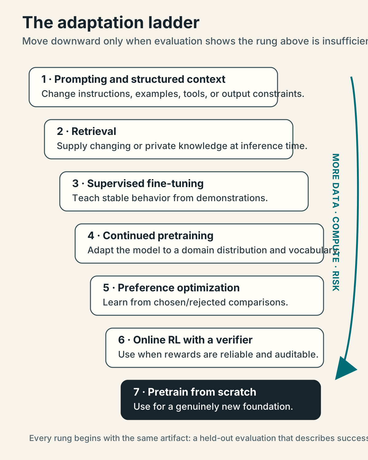
Figure 1. Cost, data requirements, and regression risk rise as you descend. This is a decision ladder, not a mandatory curriculum.
Occasional instruction failures. Start with a better prompt, examples, or constrained decoding because the desired behavior may already exist in context. Escalate only when failures persist across prompt variants and enough representative cases.
Current or private facts with citations. Start with retrieval and tools so knowledge stays inspectable and updateable. Escalate when retrieval quality is good but the model mishandles the evidence or domain language.
Arithmetic, search, database access, or execution. Start with tool use because external systems are more exact and current. Train when prompting still cannot make the model reliably select and serialize calls.
Stable tone, schema, workflow, or task mapping. Start with SFT, usually LoRA first, because demonstrations directly specify behavior. Escalate when adapter capacity is insufficient or the shift is broad.
Weak domain vocabulary and distributional fluency. Start with continued pretraining, then SFT. Raw text teaches statistical familiarity before instructions teach behavior. Proceed only when domain gains justify compute and forgetting risk.
Pairwise judgments without one perfect answer. Start with DPO or another offline preference method because chosen/rejected pairs express relative behavior. Consider online methods only after offline optimization plateaus and a reliable reward exists.
Automatically verifiable correctness. Start with rejection sampling, then possibly RL/GRPO. A verifier supplies scalable outcome feedback, but the base or SFT policy must already produce some successes.
A missing tokenizer, modality, language coverage, or broad representation. From-scratch pretraining or major architecture work may be necessary because adaptation cannot cheaply invent an absent input pathway or entire foundation. Take this rung only after proving existing foundations cannot meet the need.
Prompting, retrieval, and training are not rivals
They change different parts of the system.
- Prompting changes the evidence and instructions available for one inference.
- Retrieval changes which external information enters that inference.
- Tools let the model delegate operations and observe results.
- Training changes the conditional distribution the model implements across future inferences.
A strong application often uses all four. Fine-tuning can teach the model to query a retriever, cite returned records, and call a calculator. It does not make those components redundant.
Ask four questions before training
Is the target knowledge volatile? If yes, prefer retrieval or tools. A model checkpoint cannot issue a correction to one fact without another training cycle.
Can success be specified by examples? SFT is strongest when demonstrations are unambiguous and representative. If two competent annotators disagree, the project needs a rubric or preference data before it needs more examples.
Can success be verified? Unit tests, exact parsers, simulators, and outcome checks make rejection sampling and RL much more defensible than vibes-based rewards.
What must not regress? Name those capabilities now. “Keep the model generally smart” is not an evaluation plan.
The minimum viable experiment
Before a large run, make a table with one row per candidate system:
base model, zero/few-shot
base model + best prompt
base model + retrieval/tools
base model + LoRA SFT
base model + continued pretraining + LoRA SFT
optional preference stage
Score every row on the same frozen examples, with the same inference settings where meaningful. If retrieval already crosses the acceptance threshold, training now has to justify its extra complexity, not merely show a positive delta over a deliberately weak baseline.
Practice lens — write the stopping condition
“Train until the loss looks flat” is not a project boundary. A better boundary is: “Ship only if tool-call exact match rises from 82% to at least 94%, the 95% confidence interval excludes the baseline, general instruction-following falls by no more than two points, and p95 latency stays below 800 ms.”
2. Evaluation comes before the dataset
Most training mistakes become visible only because somebody preserved an example the optimizer never saw.
Create evaluation cases before collecting the full training corpus. Doing so forces you to define what “better” means while you are still capable of being surprised. Once you have read the test failures repeatedly and changed the data recipe in response, the test set has become a development set in practice.
Four sets, not two
For serious adaptation work, use four conceptual buckets:
| Set | Used for gradients? | Used for decisions? | Purpose |
|---|---|---|---|
| Train | Yes | Indirectly | Fit parameters |
| Development | No | Yes, repeatedly | Select data recipe, hyperparameters, and checkpoint |
| Held-out test | No | Once or rarely | Estimate performance after choices are frozen |
| Regression/control | No | Every candidate | Detect damage outside the target domain |
The regression set is the one practitioners most often omit. It may contain general writing, safety, refusal boundaries, arithmetic, coding, multilingual prompts, formatting, and representative old-domain examples. Its job is to reveal that the specialized model became less useful elsewhere.
Evaluate the system you will actually deploy
A base model evaluated with raw completion formatting is not comparable to an instruction model evaluated through its chat template. An adapter tested in BF16 can behave differently after 4-bit serving quantization. A retrieval model with gold passages is not the same system as one with a real retriever.
Pin:
- model and adapter revision;
- tokenizer revision and chat template;
- quantization and inference engine;
- system prompt and tool schemas;
- temperature, top-p, top-k, seed policy, and maximum tokens;
- retrieval corpus, embedding model, top-k, and reranker;
- evaluator version and scoring rubric.
For deterministic tasks, prefer executable graders: JSON-schema validity, unit tests, database checks, symbolic equivalence, exact normalized fields. For subjective tasks, use blinded pairwise human judgments where feasible. Model graders can help scale triage, but calibrate them against humans and keep the grader prompt/version frozen.
Public benchmarks are controls, not your product spec
EleutherAI’s evaluation harness implements many standardized tasks, and HELM emphasizes transparent evaluation across scenarios, metrics, and modalities. They are useful for broad regression checks. Neither knows what “correctly reconcile our invoice exception” means.
The highest-value eval is usually a small, carefully adjudicated set of real failures from your target workflow. Public benchmarks supplement it; they do not replace it.
A provider-neutral evaluation record
evaluation:
  name: support-tools-heldout-v1
  dataset_revision: sha256:YOUR_DATA_HASH
  split: test
  examples: 600
  grader_revision: git:YOUR_GRADER_COMMIT
  metrics:
    - tool_name_accuracy
    - arguments_exact_match
    - schema_valid_rate
    - end_to_end_task_success
  inference:
    temperature: 0.0
    max_new_tokens: 512
    chat_template_revision: tokenizer-pinned-revision
  pass_bar:
    task_success_min: 0.92
    general_regression_max_drop: 0.02
Store raw prompts, outputs, parsed scores, errors, latency, and token counts. An aggregate score without its generations is a conclusion without evidence.
3. Choose a base model like an engineer
“Use the strongest model” is incomplete advice. Strong at what? Under which template? At what precision? Licensed for which use? Able to fit in what serving budget?
Base versus instruct checkpoints
A base checkpoint is closest to the next-token pretraining objective. It is the cleaner starting point for substantial continued pretraining because it has not yet acquired a delicate chat behavior you can overwrite. It may be awkward to prompt directly.
An instruction-tuned checkpoint already follows a chat template and has undergone SFT and possibly preference optimization. It is often the efficient starting point for a modest behavioral adapter. Continuing raw-text pretraining directly on it can damage its output format, refusals, and conversational reliability; experiments have observed exactly these dimensions of forgetting in aligned models. The cited Li and Lee manuscript is an arXiv work in progress, useful as evidence rather than settled consensus. Li and Lee (2024)
A common lifecycle is therefore:
base checkpoint
  -> domain continued pretraining
  -> supervised instruction tuning
  -> optional preference or RL stage
If you begin with an instruct checkpoint because time or data is limited, mix chat-format replay examples into later training and measure the original chat behavior explicitly.
A selection scorecard
| Dimension | Questions to answer |
|---|---|
| Capability | Does the untouched model have enough reasoning, language, code, or visual competence that adaptation is plausible? |
| Modality | Text only, image input, image generation, audio, or a combination? Is the required encoder/decoder already present? |
| Size and architecture | Dense or MoE? Total versus active parameters? Context length? Does your training stack support it? |
| Memory | Can the unquantized or quantized base, activations, adapters, and optimizer state fit? |
| Ecosystem | Are tokenizer, chat template, processor, training scripts, kernels, and serving engine mature? |
| License | Can you train, redistribute adapters, serve commercially, and use outputs as intended? Are there use restrictions? |
| Provenance | Is there a model card, training/eval disclosure, and clear upstream checkpoint? |
| Serving economics | Can the adapted model meet latency and throughput goals after quantization? |
Current examples, not a leaderboard
The following are useful anchors verified on 2026-08-04. They are not a claim that one model is universally best.
Qwen3-8B-Base. A manageable dense text base with broad tooling and a useful scale for CPT and post-training experiments. The model card lists Apache-2.0.
Mistral Small 3.1 24B Base. A larger dense base from a text/vision family with a permissive ecosystem. The model card lists Apache-2.0.
Gemma 3 12B PT. Image-text input, a 128K context claim in the model card, and pretrained/instruction variants. Access is gated under Google’s Gemma terms, not Apache.
Llama 4. A large multimodal MoE family with an extensive ecosystem. Its custom Llama 4 Community License includes redistribution, attribution, scale, naming, acceptable-use, and regional multimodal terms that must be checked for the intended use.
Do not copy the word “open” from a blog post into your compliance notes. Open weights is not a license. Read the exact checkpoint’s license, acceptable-use policy, upstream dependencies, and dataset terms. Llama 4, for example, permits many uses but is governed by a custom community agreement rather than an OSI software license; the official text includes attribution, redistribution, naming, very-large-user, acceptable-use, and multimodal regional provisions. Official Llama 4 license
Likewise, a dataset tagged MIT or Apache does not automatically grant rights in every underlying record. Dataset packaging, original works, personal data, publicity rights, and contractual terms can impose separate obligations. This book offers engineering discipline, not legal advice.
The smallest sufficient base usually wins
Suppose a 7–12B model crosses your quality threshold after adaptation and a 70B model gains three additional points. The larger model may need an expensive multi-GPU serving replica forever. Training cost happens once; inference cost repeats.
Choose by quality at an acceptable total cost, not quality alone:
This is why distillation, smaller bases trained on more relevant examples, and retrieval-backed systems can beat a superficially “more powerful” checkpoint as products.
4. What renting a GPU actually means
A cloud GPU is not a magical cuda device floating on the internet. You rent a machine—or part of one—with GPUs, CPU RAM, storage, networking, an operating system or container, and a billing clock.
The practical lifecycle is:
choose region and GPU
  -> provision instance/container
  -> attach persistent storage
  -> install a pinned environment
  -> copy or stream versioned data
  -> run a tiny end-to-end smoke test
  -> benchmark tokens/second and peak VRAM
  -> launch resumable training
  -> copy checkpoints and logs off the instance
  -> verify artifacts
  -> terminate compute and unneeded disks
Three provider shapes
GPU-specialist clouds such as Runpod and Lambda tend to make a single GPU or small node easier to acquire. Their product surface is narrower than a hyperscaler, and prices can be attractive. Capacity and machine consistency still vary.
Hyperscalers such as AWS and Google Cloud provide mature identity, networking, object storage, monitoring, quotas, and managed services. They can cost more and require more setup. Their reservation and spot products are useful when you understand them.
Marketplaces such as Vast.ai aggregate third-party hosts. Prices are dynamic and interruptible listings can be much cheaper, but reliability, bandwidth, storage behavior, security posture, and interconnect vary by host. Vast’s official documentation explicitly describes a live marketplace rather than static prices and notes that storage continues billing on stopped instances. Vast pricing model
Current price snapshot
The figures below were checked against official pages on 2026-08-04. They are USD before taxes, and they compare named products rather than promising availability. The stacked layout is intentional: narrow Kindle screens should not have to shrink a four-column pricing table into illegibility.
Runpod Pods, Community Cloud
- H100 SXM 80GB: $2.99 per GPU-hour.
- H100 PCIe 80GB: $2.89 per GPU-hour.
- A100 PCIe 80GB: $1.39 per GPU-hour.
- L40S 48GB: $0.99 per GPU-hour.
- Boundary: dedicated Pod listings; host and availability vary, and storage is priced separately.
Lambda self-serve, one-GPU instances
- H100 PCIe 80GB: $3.29 per instance-hour.
- A6000 48GB: $1.09 per instance-hour.
- Boundary: on-demand, first-come capacity; the listed instance bundle includes its stated CPU, RAM, and storage.
Lambda self-serve, eight-GPU instance
- Eight H100 SXM GPUs: 31.92 per node-hour.
- Boundary: on-demand, first-come capacity; budget the whole eight-GPU node and verify availability.
AWS EC2 Capacity Blocks for ML
p5.4xlarge, one H100, US East (Ohio or N. Virginia): $5.191 per reserved instance-hour.p5.48xlarge, eight H100s, US East (Ohio or N. Virginia): **5.191 per accelerator-hour.- Boundary: this is an advance reservation, not ordinary on-demand or Spot capacity. AWS charges the reservation fee up front for every hour in the purchased block, whether or not your training process uses every reserved hour. Operating-system fees can be additional, and the reservation cannot be canceled after purchase. Searches specify 1-day increments through 14 days and 7-day increments thereafter. Because blocks end at 11:30 UTC, AWS may return offers slightly shorter or longer than the requested duration; the displayed offer duration and total price are authoritative. AWS purchase documentation
Google Cloud Spot, Iowa (us-central1)
a3-highgpu-1g, one H100: approximately $6.3262 per interruptible instance-hour.- Boundary: this is the bundled accelerator-optimized VM price shown for one GPU, 26 vCPUs, 234 GiB memory, and 750 GiB local SSD—not the GPU component alone. Spot capacity can be reclaimed and the current rate can change.
Sources: Runpod, Lambda, AWS Capacity Blocks, and Google Spot. Recheck the exact region, machine, reservation duration, storage, and operating-system terms immediately before purchase.
On-demand versus interruptible
Use interruptible capacity only when the job can resume.
A resumable job needs:
- checkpoints on storage that survives the worker;
- model, optimizer, scheduler, scaler, RNG, data-cursor, and step state;
- idempotent startup that detects the newest complete checkpoint;
- checkpoint intervals shorter than the amount of recompute you are willing to lose;
- graceful termination handling when the provider offers notice;
- periodic artifact copies to independent object storage.
For deployment, adapter weights can be sufficient only together with the exact accessible base checkpoint, tokenizer or processor, adapter configuration, chat template, and pinned revisions. For resuming Adam halfway through an epoch, adapter weights alone are not sufficient; preserve optimizer, scheduler, RNG, scaler, and data state too.
A provider-neutral project layout
project/
  configs/
    train.yaml
    eval.yaml
  data/
    MANIFEST.json
  src/
    prepare.py
    train.py
    evaluate.py
  tests/
  requirements.lock
  README.md

persistent-volume/
  datasets/<dataset-hash>/
  checkpoints/<run-id>/
  logs/<run-id>/
  exports/<run-id>/
Keep secrets out of the image and repository. Pass read-only dataset/model credentials through the provider’s secret mechanism. Use a private network or strict firewall, and do not place sensitive training data on an arbitrary marketplace host without a security and contractual review.
The first 30 minutes on a rented machine
- Record GPU model, count, driver, CUDA runtime, CPU RAM, disk, and network mount.
- Install from a lockfile or immutable container digest.
- Download one small shard and one model shard.
- Decode ten examples and inspect them manually.
- Run one training step, one evaluation step, one checkpoint save, and one resume.
- Measure peak allocated/reserved VRAM and tokens per second after warm-up.
- Extrapolate runtime and cost from that measurement.
- Set a billing alert and an automatic termination condition.
The cloud rule that saves the most money
A stopped training process does not necessarily mean a stopped bill. Delete or terminate idle compute deliberately, and know which disks, IPs, snapshots, and object-store artifacts continue to incur charges.
Checkpoint quiz I — choose before you train
1. You need answers from policies that change weekly and must cite the operative paragraph. What is the best first intervention?
- A. Full fine-tuning on last week’s policies
- B. Retrieval with versioned policy documents and citations
- C. Preference optimization
- D. A larger tokenizer
2. Why is an instruction checkpoint a delicate starting point for raw-text continued pretraining?
- A. It has no tokenizer.
- B. Raw next-token updates can erode chat formatting and alignment behavior learned in post-training.
- C. Instruction models cannot compute gradients.
- D. Continued pretraining always changes the architecture.
3. A marketplace lists an H100 at a low hourly price. Which cost is safe to infer immediately?
- A. The complete training budget
- B. Lifetime serving cost
- C. GPU-hour cost only; storage, bandwidth, reliability, and runtime still need measurement
- D. The number of examples required
4. Why make a held-out set before collecting all training examples?
- A. So it can be copied into the training set later
- B. To define success before repeated error analysis contaminates the test
- C. Because optimizers require a test tensor
- D. To increase GPU utilization
Answers appear near the end of the book.
Part II — Make the run fit
5. GPU memory without folklore
“Will a 7B model fit?” is not answerable until you say for what operation, at what precision, with what sequence length and optimizer.
Inference mostly needs weights and a KV cache. Training also needs gradients, optimizer states, saved activations, temporary workspaces, and sometimes a full-precision master copy. Parameter-efficient training freezes most weights and removes most gradient/optimizer storage, but it still performs forward and backward computation through the base.
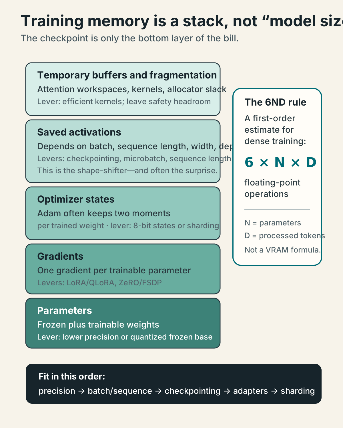
Figure 2. “Will the model fit?” is really a question about the entire stack for a particular operation, precision, batch, and sequence length.
Weight memory is the easy part
For parameters stored at bytes each:
Ignoring quantization metadata and allocator overhead:
| Model size | BF16/FP16, 2 bytes | INT8, about 1 byte | INT4, about 0.5 byte |
|---|---|---|---|
| 1B | 2 GB | 1 GB | 0.5 GB |
| 8B | 16 GB | 8 GB | 4 GB |
| 24B | 48 GB | 24 GB | 12 GB |
| 70B | 140 GB | 70 GB | 35 GB |
Real quantized formats store scales, zero points, alignment padding, and sometimes higher-precision exceptions. Treat the table as a lower-bound intuition, then measure the actual checkpoint and runtime.
Think in memory and topology tiers
GPU names are less useful than the memory and interconnect constraints they imply. As rough experiment categories—not fit guarantees:
- 24GB class: small-model full tuning or roughly 7B–8B LoRA/QLoRA at controlled sequence and microbatch sizes. Long contexts, VLM image tokens, and optimizer variants can exhaust it quickly.
- 48GB class: more room for 7B–14B adapter work, longer contexts, larger batches, and many image-generator LoRAs. Full-parameter Adam on an 8B model still does not fit merely because the weights do.
- 80GB class: comfortable headroom for many 8B adapter and VLM experiments, larger quantized bases, or one shard of full training. It is not automatically enough for an unsharded 8B full fine-tune once optimizer state and activations are included.
- Multi-GPU SXM/NVLink class: the natural category for sharded full tuning, larger continual-pretraining runs, and communication-heavy workloads. Budget for the whole node and verify topology; several unrelated PCIe GPUs are not interchangeable with one high-bandwidth SXM node.
The honest sizing procedure remains: load the exact revision, run the exact processor and sequence shape, take one optimizer step, and measure peak reserved memory.
Why full fine-tuning is much larger
A common mixed-precision AdamW accounting per trainable parameter is roughly:
BF16 model weight          2 bytes
BF16 gradient              2 bytes
FP32 master weight         4 bytes
FP32 Adam first moment     4 bytes
FP32 Adam second moment    4 bytes
                         --------
                           16 bytes
Implementations differ. Some keep gradients in FP32, some avoid a separate master weight, fused optimizers pack state differently, and frameworks create transient buffers. But is a useful planning floor for unsharded mixed-precision Adam before activations.
For an 8B model, that is about 128 GB of model state, not counting activations. The same checkpoint that performs inference on one 24GB or 48GB GPU after quantization may require several 80GB GPUs to full-fine-tune comfortably.
Activations are the shape-shifter
Activation memory grows with microbatch size , sequence length , width , and layers . A simplified view is:
Naive attention also materializes structures proportional to per head. Memory-efficient attention kernels avoid storing the full score matrix, but the computation still gets more expensive as context grows.
This explains a common surprise: a model fits at 1,024 tokens and fails at 8,192 even though its parameter count did not change.
The knobs and what they really trade
Mixed precision stores/computes many tensors in BF16 or FP16. BF16 usually has a friendlier exponent range when the hardware supports it. Neither means every tensor is low precision.
Microbatch size is the examples processed simultaneously on each GPU. Reducing it saves activation memory but may reduce utilization.
Gradient accumulation runs several microbatches before an optimizer update. It recovers a larger effective batch without holding all activations at once. It does not create the communication or throughput behavior of a genuinely larger parallel batch.
Activation checkpointing saves selected activations and recomputes them during backward. It trades extra FLOPs and wall time for memory. This is unrelated to saving a training checkpoint to disk.
Sequence packing fills training rows with real tokens instead of padding. It can dramatically improve useful tokens per second, provided document boundaries and attention/loss masks are correct.
Flash/memory-efficient attention changes how attention is computed and tiled so the full matrix need not reside in high-bandwidth memory.
CPU/NVMe offload moves states away from the GPU. It can make an otherwise impossible run fit, but PCIe and storage transfers may make it painfully slow.
Effective batch and number of updates
If every row has non-padding tokens processed, then:
where is GPU count, is microbatch sequences per GPU, and is gradient-accumulation steps.
Example:
4 GPUs
2 sequences/GPU
2048 non-padding tokens/sequence
8 accumulation steps

tokens/update = 4 * 2 * 2048 * 8 = 131,072
If the epoch contains 131 million non-padding tokens, it has about 1,000 optimizer updates. Log processed and supervised tokens, not only epochs: packing efficiency, masking, and example lengths make “three epochs” incomparable across datasets.
Data parallelism, FSDP, and ZeRO
Ordinary distributed data parallelism replicates the model on each GPU, gives each rank different examples, and averages gradients. It accelerates throughput but does not solve model-state memory because every rank holds a copy.
DeepSpeed ZeRO partitions increasingly more state:
- Stage 1 partitions optimizer states.
- Stage 2 also partitions gradients.
- Stage 3 also partitions model parameters and gathers them as needed.
PyTorch FSDP similarly shards parameters, gradients, and optimizer state according to its configuration. These systems make total cluster memory available to one logical model, at the cost of communication, configuration complexity, and more intricate checkpointing.
They do not make slow interconnect disappear. Eight isolated PCIe GPUs on separate weakly connected hosts are not equivalent to eight SXM GPUs with high-bandwidth intra-node links. For multi-GPU training, topology can matter as much as the name printed on the accelerator.
A practical optimization order
When a run OOMs:
- Confirm the failure is GPU memory, not host RAM or disk.
- Reduce microbatch size.
- Enable mixed precision appropriate to the GPU.
- Enable gradient/activation checkpointing.
- Use memory-efficient attention and packing.
- For adaptation, choose LoRA or QLoRA if scientifically acceptable.
- Shard with FSDP or ZeRO.
- Offload only after understanding the throughput penalty.
- Reduce context length or choose a smaller base if the product allows it.
Do not begin by combining every trick. Change one layer of complexity at a time and rerun the checkpoint-resume test.
6. Turn tokens into hours and dollars
The most reliable cost estimate comes from a short representative pilot on the exact stack. Its denominator is all non-padding tokens processed by the forward/backward pass, not only tokens whose labels contribute to the loss:
For assistant-only SFT, therefore, record two counters. Processed tokens include prompt and assistant tokens that occupy compute; supervised tokens are the assistant tokens with non-masked labels. The second counter describes learning-signal density, but the first predicts runtime. Then add headroom, storage, downloads, evaluation generation, failed runs, and idle setup time.
Why FLOP estimates still help
For a dense decoder trained with a standard next-token objective, a widely used first approximation is:
where is parameter count and is training tokens. It is an order-of-magnitude model, not a bill: architecture, sequence length, attention implementation, sparsity, recomputation, padding, and hardware utilization all move the result.
If one GPU sustains useful training FLOPs/second and multi-GPU scaling efficiency is :
Use this before provisioning; replace it with measured token throughput after the smoke benchmark.
All hours and subtotals below are rounded planning estimates, not quotes. For AWS, each fractional-hour figure is a continuous-use equivalent retained only to compare hourly rates. It is never the purchasable bill. The paired reservation figure rounds planning duration up to the next nominal 1-day or 7-day increment. AWS can return an offer slightly shorter or longer because blocks share an 11:30 UTC end time, so the offer’s displayed duration and prepaid, noncancelable price always override this planning floor. Purchase rules
Worked budget A — 8B QLoRA SFT
Suppose you have 50,000 packed examples averaging 1,000 non-padding tokens processed per example and train three epochs. Separately, suppose 650 of those 1,000 tokens are assistant targets on average:
processed tokens  = 50,000 * 1,000 * 3 = 150,000,000
supervised tokens = 50,000 *   650 * 3 =  97,500,000
Assume—not claim—that the exact QLoRA configuration measures 7,000 aggregate processed non-padding tokens/second on one H100. Add 25% headroom:
raw hours ≈ 150,000,000 / 7,000 / 3,600 ≈ 5.95
planned hours ≈ 5.95 * 1.25 ≈ 7.44
At prices verified 2026-08-04:
| Product | Arithmetic | Usage-duration estimate |
|---|---|---|
| Runpod H100 PCIe | 7.44 × $2.89 | ≈$21.50 |
| Lambda H100 PCIe | 7.44 × $3.29 | ≈$24.48 |
| AWS p5.4xlarge hourly-rate comparison | 7.44 × $5.191 | ≈$38.62 equivalent |
The AWS comparison is not purchasable as 7.44 hours. A nominal one-day planning floor is 24 hours × 124.58 prepaid**. Use the exact duration and price of the returned offer.
This excludes storage, tax, data transfer, environment setup, eval inference, and failed experiments. The important lesson is not “QLoRA costs $21.” It is that once a pilot exposes throughput, the estimate becomes simple arithmetic and may be much smaller than the engineering labor around it.
Worked budget B — full SFT across eight H100s
Use the same 150M tokens. Suppose a representative pilot measures 22,000 aggregate tokens/second after communication and checkpointing, and you reserve 30% headroom:
hours ≈ 150,000,000 / 22,000 / 3,600 * 1.30 ≈ 2.46| Product | Arithmetic | Usage-duration estimate |
|---|---|---|
| Runpod 8 × H100 SXM | unrounded hours × 8 × $2.99 | ≈$58.89 |
| Lambda 8 × H100 SXM | unrounded hours × 8 × $3.99 | ≈$78.59 |
| AWS p5.48xlarge hourly-rate comparison | unrounded hours × $41.528 | ≈$102.25 equivalent |
The AWS comparison is not purchasable as 2.46 hours. A nominal one-day planning floor is 24 hours × 996.67 prepaid**. Use the exact duration and price of the returned offer.
Do not infer that full SFT is only three times the QLoRA bill. This assumed multi-GPU job may not be available, and its setup, data pipeline, sharded checkpointing, and retries are more complex. Full tuning also produces a complete new checkpoint rather than a small adapter and often demands more hyperparameter care.
Worked budget C — 7B continued pretraining on 5B tokens
Assume a dense 7B model, 5B tokens, eight H100s, 300 TFLOP/s sustained useful training throughput per GPU, and 85% scaling efficiency:
FLOPs = 6 * 7e9 * 5e9 = 2.1e20
hours = 2.1e20 / (8 * 300e12 * 0.85) / 3,600
= 28.59 hours| Product | Arithmetic | Usage-duration estimate |
|---|---|---|
| Runpod 8 × H100 SXM | unrounded hours × 8 × $2.99 | ≈$683.99 |
| Lambda 8 × H100 SXM | unrounded hours × 8 × $3.99 | ≈$912.75 |
| AWS p5.48xlarge hourly-rate comparison | unrounded hours × $41.528 | ≈$1,187.48 equivalent |
The 28.59-hour AWS comparison requires at least a nominal two-day planning window: 48 hours × 1,993.34 prepaid**. Use the exact duration and price of the returned offer.
That is one candidate run. Add pilots, ablations, checkpoint storage, validation, and failure margin. A realistic project budget might be several times the clean compute subtotal.
Worked budget D — the from-scratch reality check
The Chinchilla paper’s memorable compute-optimal planning point is roughly 20 training tokens per parameter for a dense model under its assumptions. Hoffmann et al.
A 7B model would therefore suggest about 140B tokens:
FLOPs = 6 * 7e9 * 140e9 = 5.88e21
hours on the same assumed 8-H100 setup = 800.65
elapsed time = about 33.4 days
Runpod compute subtotal = unrounded hours * 8 * $2.99 ≈ $19,151.63
Lambda compute subtotal = unrounded hours * 8 * $3.99 ≈ $25,556.86
AWS continuous-use equivalent = unrounded hours * $41.528 ≈ $33,249.54
AWS nominal 35-day planning floor = 840 hours * $41.528 ≈ $34,883.52 prepaid
The AWS duration rounds approximately 33.36 days up to five weeks because searches beyond 14 days use 7-day increments. It remains a planning floor rather than a quote: the returned offer can be slightly shorter or longer, and its displayed prepaid price is authoritative.
These optimistic arithmetic examples omit data acquisition/processing, tokenizer experiments, evaluation, engineering time, idle capacity, failed runs, and the fact that one eight-GPU node may not sustain the assumed throughput continuously. They do show the cliff between adapting a 7B checkpoint and creating a competitive 7B foundation.
A 100M-parameter educational model at 2B tokens is different:
FLOPs = 6 * 100e6 * 2e9 = 1.2e18
idealized time at 120 TFLOP/s sustained ≈ 2.78 GPU-hours
Overheads dominate at that scale, but the experiment is accessible and can teach tokenization, schedules, scaling, checkpoints, and evaluation. Its purpose is understanding, not frontier capability.
A budget sheet that admits uncertainty
budget:
  verified_date: 2026-08-04
  model_parameters: 8_000_000_000
  processed_nonpadding_tokens_including_epochs: 150_000_000
  supervised_target_tokens_including_epochs: 97_500_000
  pilot:
    gpu: H100-80GB
    aggregate_tokens_per_second: 7000
    warmup_steps_excluded: 20
    sequence_length: 2048
  planned_hours_raw: 5.95
  headroom_fraction: 0.25
  planned_hours: 7.44
  price_per_gpu_hour_usd: 2.89
  gpu_count: 1
  compute_subtotal_usd_estimate: 21.50
  exclusions:
    - persistent_storage
    - network_egress
    - evaluation
    - taxes
    - failed_runs
Cost traps
- Comparing H100 prices without distinguishing PCIe from SXM or one GPU from an 8-GPU node.
- Assuming eight GPUs make the job eight times faster.
- Counting raw examples or supervised targets instead of all processed non-padding tokens.
- Ignoring evaluation generation, which can dominate RL and best-of- pipelines.
- Leaving a notebook instance alive overnight.
- Downloading a multi-hundred-gigabyte checkpoint repeatedly instead of caching it on a controlled volume.
- Saving every checkpoint forever.
- Choosing cheap GPUs whose weak interconnect makes distributed training slower and more expensive overall.
Part III — Manufacture the data
7. A dataset is a designed artifact
The training loop never sees “our domain” or “the web.” It sees serialized, tokenized examples produced by a pipeline of choices.

Those choices include source eligibility, extraction, filtering, language detection, personal-data removal, deduplication, labeling, formatting, mixing, splitting, tokenization, packing, and loss masking. Each can improve a benchmark while silently breaking another property.
Start from the learning signal
Different stages require different records.
| Stage | Minimal record | What the loss teaches |
|---|---|---|
| Continued pretraining | {"text": ...} | Predict the next token in the target distribution |
| Prompt-completion SFT | prompt, completion | Produce this completion after this prompt |
| Conversational SFT | ordered messages with roles | Follow the chat protocol and imitate assistant turns |
| Tool-use SFT | messages, tool schemas, tool calls/results | Select and serialize calls in context |
| DPO | prompt, chosen response, rejected response | Increase relative probability of the preferred response |
| Reward modeling | prompt, candidate responses, ranks/scores | Predict a preference signal |
| Verifiable RL | prompts plus executable reward/verifier | Find outputs that maximize measured outcomes |
| VLM SFT | images plus messages/answers | Map visual evidence and text context to target text |
| Text-to-image adaptation | images, captions, optional masks/conditioning | Associate visual patterns with text or control inputs |
Do not convert raw manuals into fake question-answer pairs unless the target really is answering those questions and the generated answers are verified. Continued pretraining can ingest raw prose; SFT needs demonstrations of behavior.
Provenance is a first-class feature
For every record or source shard, retain enough metadata to answer:
- Where did it come from?
- Under what license or permission was it acquired?
- When was it captured, and what version?
- Which transformations were applied?
- Does it contain a person, customer, secret, or regulated field?
- Can it be removed later?
- Which split and sampling weight received it?
At minimum, a manifest might contain:
{
  "dataset_id": "support-actions-v3",
  "content_sha256": "...",
  "schema_version": 3,
  "sources": [
    {
      "name": "resolved_tickets",
      "snapshot": "2026-07-15",
      "permission_basis": "internal-approved-use",
      "records_in": 81422,
      "records_out": 51709
    }
  ],
  "filters": ["secret_scan_v2", "pii_redaction_v4", "language_en_v1"],
  "dedup": {"method": "normalized_minhash", "threshold": 0.85},
  "split_unit": "customer_case_id",
  "train_records": 45000,
  "dev_records": 3200,
  "test_records": 3509
}
If you cannot delete one person’s data without rebuilding the corpus from mystery scripts, the pipeline is not ready for sensitive data.
Availability is not permission
Publicly reachable content can still be copyrighted, contractually restricted, private in context, or subject to publicity and data-protection rights. A dataset card can license the collection or metadata while underlying works retain their own terms.
FineWeb, for example, publishes a reproducible cleaned/deduplicated Common Crawl pipeline and lists ODC-By 1.0, while its card also points to Common Crawl terms and documents harmful-content limitations.
The Stack v2 is especially easy to misunderstand. Its Hub rows primarily expose Software Heritage identifiers and provenance—such as blob_id, content_id, repository directory/snapshot/revision IDs, path, crawl date, and detected license metadata—not a convenient self-contained dump of every code file. File bodies live in Software Heritage-backed storage. Bulk content access requires an agreement with Software Heritage and INRIA plus configured credentials; accepting the gated Hub terms also shares account contact information with the maintainers. The terms require users to follow original code licenses, preserve applicable attribution, adhere to Software Heritage’s model-training principles, and update local copies as validated removal requests are enacted. License detection can be wrong, and the corpus may contain secrets, personal data, or malicious code. Preserve the SWH IDs through filtering and training so a generated-code audit or removal rebuild remains possible.
For commercial or sensitive work, have counsel or the responsible governance function approve the recipe. Record the decision, not just the URL.
Split by the unit that can leak
Random row splitting is often wrong.
- Split support tickets by customer case or conversation, not message.
- Split code by repository, not file or function.
- Split documents before chunking or packing.
- Split medical data by patient, not scan.
- Split images by subject/session/photographer when those correlations matter.
- Split temporal forecasting data by time.
Near-duplicate eval contamination is still contamination. Hash normalized text for exact matches, use MinHash/LSH or embeddings for near-duplicates, and inspect the closest cross-split pairs manually.
Quality beats indiscriminate volume in post-training
One contradictory or malformed SFT example can supply thousands of token-level gradients in the wrong direction. Build automatic gates:
- schema validity and required roles;
- nonempty, bounded lengths;
- valid tool names/arguments;
- executable code/tests where applicable;
- citation support for factual answers;
- no secret tokens or personal identifiers;
- no assistant answer leaked into the prompt;
- no duplicate prompts with incompatible answers;
- language and encoding checks;
- per-source and per-category distributions.
Then sample manually from every source, length bucket, task category, and filter boundary—not merely random rows from the dominant source.
8. Where useful data actually comes from
There is no universal “best fine-tuning dataset.” The closest match to the deployed input distribution and success criterion is usually the valuable one.
A discovery map
General or domain continued pretraining. Start with your licensed corpus, FineWeb samples, applicable Wikipedia/Wikimedia text, or papers with compatible licenses. You still need source filtering, domain weighting, deduplication, PII review, split-contamination checks, and tokenizer analysis.
Code. Start with repositories you may use, The Stack v2 under its access/provenance terms, or generated tasks backed by tests. You still need license and attribution review, secret/malware scanning, repository-level splits, and executable validation.
Human instruction following. Start with your task demonstrations or OASST1, whose card describes Apache-2.0 multilingual human feedback. You still need to convert trees carefully, filter quality, and match the intended task distribution.
Preference learning. Start with blinded labels from your users or carefully inspected public sets such as Anthropic HH-RLHF and UltraFeedback Binarized. You still need license review, ties, prompt-contamination checks, and controls for synthetic-judge bias.
Classification and extraction. Start with adjudicated business labels or public task data with explicit terms. Preserve class priors and hard negatives, and convert to generative form only if the serving interface needs it.
Math and reasoning. Start with licensed problem sets, generated problems with verifiers, or safe proof/code environments. Separate templates across splits, check answer equivalence, and avoid benchmark leakage.
Tool and agent behavior. Start with consented successful traces, corrected failures, or simulated tasks in sandboxes. Preserve tool versions and outcomes; never promote an unverified self-generated trajectory merely because it looks fluent.
VLM understanding. Start with your image-document pairs, purpose-built screenshots/forms, or COCO and Visual Genome after term review. Check image rights, faces/PII, OCR leakage, image-family splits, and whether answers are visibly grounded.
Image generation. Prefer consented first-party, commissioned, or licensed images; per-file-compatible Wikimedia Commons material can also help. Research corpora such as DataComp require purpose-specific review. Captions, creator and subject consent, trademarks, identity/style risk, removal, and attribution remain your work.
The Hugging Face Hub is a discovery mechanism, not a due-diligence substitute. Read the dataset card, source paper, license file, discussions, upstream terms, and actual sample content. Pin a revision instead of loading mutable main forever.
Human, synthetic, and operational data
Human-authored data can express nuance and original expertise but is expensive and inconsistent. Use rubrics, calibration rounds, double labels on a subset, disagreement tracking, and adjudication.
Synthetic data is useful for coverage, transformations, adversarial variants, and tasks with executable verification. It also copies the teacher’s biases and may create polished but false supervision. Keep the teacher/model/prompt revision and verifier outcome per record.
Operational data best matches reality, but it contains privacy, consent, selection, and feedback-loop hazards. “Resolved ticket” does not mean “excellent answer”; a human may have repaired it later. Train on outcomes only after reconstructing what actually succeeded.
Dataset mixture as a curriculum
Let source have sampling weight , with . The expected training distribution is:
The weights are an implicit product decision. If 70% of SFT tokens are code, the model receives more code gradients even if “code” is only 10% of rows. Track both record and token proportions.
Temperature sampling can prevent a huge source from swallowing smaller ones:
where is source size. This is a starting heuristic, not a substitute for measuring per-domain gains and regressions.
A streaming inspection snippet
from datasets import load_dataset

stream = load_dataset(
    "HuggingFaceFW/fineweb",
    name="sample-10BT",
    split="train",
    streaming=True,
    revision="PIN_A_COMMIT_OR_TAG",
)

for index, row in enumerate(stream.take(20)):
    text = row["text"]
    print(index, len(text), repr(text[:240]))
Streaming is excellent for inspection. A high-throughput run usually wants versioned local shards, pretokenization, sequential reads, and checksums so training is not coupled to an external service.
Validators worth running before every launch
Text conversations and VLM conversations have different schemas. Validate them separately, and raise ordinary exceptions rather than relying on assert, which Python can disable with optimization flags.
For text-only conversational SFT:
import json
from collections import Counter
from pathlib import Path

ALLOWED_ROLES = {"system", "user", "assistant", "tool"}


def require(condition: bool, line_number: int, message: str) -> None:
    if not condition:
        raise ValueError(f"line {line_number}: {message}")


def validate_text_jsonl(path: str) -> None:
    counts = Counter()
    seen_ids = set()

    with Path(path).open(encoding="utf-8") as source:
        for line_number, line in enumerate(source, start=1):
            row = json.loads(line)
            row_id = row.get("id")
            require(isinstance(row_id, str) and row_id, line_number, "bad id")
            require(row_id not in seen_ids, line_number, "duplicate id")
            seen_ids.add(row_id)

            messages = row.get("messages")
            require(
                isinstance(messages, list) and messages,
                line_number,
                "bad messages",
            )
            require(
                all(isinstance(message, dict) for message in messages),
                line_number,
                "messages must contain objects",
            )
            require(messages[-1].get("role") == "assistant", line_number, "last role")
            for message in messages:
                require(message.get("role") in ALLOWED_ROLES, line_number, "bad role")
                content = message.get("content")
                require(
                    isinstance(content, str) and content.strip(),
                    line_number,
                    "bad text",
                )

            counts[row.get("source", "unknown")] += 1

    print("records", len(seen_ids))
    print("sources", counts)
For a VLM JSONL manifest whose images field still contains paths:
import json
from pathlib import Path


def validate_vlm_jsonl(path: str, image_root: str) -> None:
    root = Path(image_root).resolve()
    with Path(path).open(encoding="utf-8") as source:
        for line_number, line in enumerate(source, start=1):
            row = json.loads(line)
            images = row.get("images")
            if not isinstance(images, list) or not images:
                raise ValueError(f"line {line_number}: images must be a nonempty list")
            if not all(isinstance(item, str) and item for item in images):
                raise ValueError(f"line {line_number}: image paths must be strings")

            resolved = [(root / item).resolve() for item in images]
            try:
                for item in resolved:
                    item.relative_to(root)
            except ValueError as error:
                raise ValueError(
                    f"line {line_number}: image escapes image_root"
                ) from error
            missing = [str(item) for item in resolved if not item.is_file()]
            if missing:
                raise ValueError(f"line {line_number}: missing images: {missing}")

            messages = row.get("messages")
            if not isinstance(messages, list) or not messages:
                raise ValueError(f"line {line_number}: bad messages")
            if not all(isinstance(message, dict) for message in messages):
                raise ValueError(f"line {line_number}: messages must contain objects")
            if messages[-1].get("role") != "assistant":
                raise ValueError(f"line {line_number}: last role must be assistant")

            parts = []
            for message in messages:
                content = message.get("content")
                if not isinstance(content, list):
                    raise ValueError(f"line {line_number}: VLM content must be a list")
                if not all(isinstance(part, dict) for part in content):
                    raise ValueError(f"line {line_number}: malformed VLM content")
                parts.extend(content)
            placeholders = sum(part.get("type") == "image" for part in parts)
            if placeholders != len(images):
                raise ValueError(f"line {line_number}: image placeholder mismatch")
Real validation should also detect secrets/PII, compute token lengths with the exact tokenizer and processor, enforce tool schemas, compare cross-split hashes, check image decode and dimensions, and emit a machine-readable report. The point is to make “the file loaded” the beginning of validation, not the end.
9. Experiment tracking is part of the model
A checkpoint without its lineage is an anecdote.
For every run, record:
- git commit and dirty-state diff;
- container digest and library lock;
- model/tokenizer/processor revisions;
- dataset manifest hash and mixture weights;
- all hyperparameters, seeds, and precision settings;
- GPU type/count/topology and provider product;
- trainable and total parameter counts;
- peak VRAM, processed non-padding tokens/second, supervised target-token count, wall time, and cost;
- train/dev metrics by category over steps;
- raw evaluation generations and error labels;
- checkpoint inventory and final export hash.
MLflow Tracking is one open system for logging parameters, code versions, metrics, artifacts, and dataset inputs. Weights & Biases and other systems can fill the same role. The tool matters less than the invariant: another person should be able to identify exactly what changed between two curves.
Make the first matrix small
Do not begin with a 40-run sweep. Start with the largest scientific contrasts:
base vs adapter
low vs moderate learning rate
without vs with replay mixture
one epoch vs checkpoint selected by dev metric
Use identical seeds only where the comparison benefits from paired noise; run multiple seeds when variance could change the conclusion. A tiny dev set with a noisy model grader can make hyperparameter search optimize grader noise.
Save by evidence, not habit
Useful checkpoints are:
- before any update;
- after the smoke test;
- at fixed token intervals;
- when the predeclared dev metric improves;
- at the end;
- before changing stage or data mixture.
Evaluate more than the final checkpoint. Target performance may peak before general regression accelerates.
Checkpoint quiz II — memory, cost, and data
5. Why can an 8B checkpoint fit for quantized inference but fail during full fine-tuning on the same GPU?
- A. Training uses a different tokenizer alphabet.
- B. Gradients, optimizer states, master weights, activations, and workspaces add far more memory than quantized inference weights.
- C. Eight billion is an inference-only parameter count.
- D. Backpropagation disables GPU memory.
6. A pilot measures 5,000 aggregate processed non-padding tokens/s and the planned run has 180M such tokens. Before headroom, runtime is closest to:
- A. 1 hour
- B. 10 hours
- C. 100 hours
- D. 1,000 hours
7. Why split code by repository rather than file?
- A. Optimizers require one repository per batch.
- B. Related and duplicated files from the same project can otherwise leak across train and test.
- C. Repository names improve tokenization.
- D. It guarantees every license is permissive.
8. What does QLoRA primarily save relative to full fine-tuning?
- A. It deletes the tokenizer.
- B. It stores the frozen base in 4-bit form and trains small adapters, greatly reducing model-state memory.
- C. It avoids all forward computation through the base.
- D. It makes sequence length irrelevant.
Part IV — Change the language model
10. Supervised fine-tuning: teach behavior by demonstration
Pretraining teaches a model to continue text from a broad distribution. Supervised fine-tuning teaches a narrower conditional behavior:
When the context looks like this, produce an answer shaped like that.
For a sequence of tokens , ordinary causal loss is:
In instruction SFT, we often mask the user/system/tool-input tokens and calculate loss only on tokens the assistant should generate. With a binary mask :
This distinction matters. If you train equally on user prompts, you ask the model to imitate both sides of the conversation. For a conversational messages dataset, this is assistant-only loss; for a prompt-completion dataset, the analogous setting is completion-only loss. Either usually better matches a deployed assistant than full-sequence loss, although training on the full transcript can be appropriate for base-model adaptation or particular protocols.
The chat template is part of the model
A structured conversation:
{
  "messages": [
    {"role": "system", "content": "You classify support requests."},
    {"role": "user", "content": "My card was charged twice."},
    {"role": "assistant", "content": "billing.duplicate_charge"}
  ]
}
must become one token stream. A template may insert beginning/end tokens, role markers, separators, and generation prompts:
<bos><system>You classify support requests.</system>
<user>My card was charged twice.</user>
<assistant>billing.duplicate_charge</assistant><eos>
Different model families expect different control tokens. Reusing a template from another family can create a dataset that looks correct as JSON and is wrong as tokens.
Before training, print:
- the structured example;
- the exact rendered text;
- token IDs and decoded tokens;
- the loss mask;
- the truncation result.
Ensure the first assistant token is included in the loss, user tokens are masked as intended, EOS is present, and truncation did not remove the answer while retaining the question.
SFT is especially good at
- stable formats and schemas;
- tone, brevity, and workflow conventions;
- classification/extraction expressed as generation;
- tool selection and call serialization;
- teaching when to abstain or ask for missing information;
- converting domain evidence into the desired answer style;
- compressing many prompt examples into weights to reduce prompt length.
It is less reliable as a way to insert a large, updateable fact database. It can teach a fact from repeated examples, but the result is hard to update, cite, or guarantee.
Coverage before volume
Suppose 80% of real requests are easy category A and 5% are dangerous category D. Mirroring production frequencies exactly may leave D undertrained. Oversampling D may protect it but distort the model’s prior.
Do not jump from zero to a 30,000-example labeling project. Use progressive evidence gates:
- 300–500 demonstrations: cover every declared behavior and failure mode, validate templates/masks, overfit a tiny subset, and run the first held-out task evaluation.
- 1,000–2,000 demonstrations: repair the error taxonomy, measure whether another example category actually moves its slice, and compare against the prompting/retrieval baseline.
- 10,000–30,000 only after the curve earns it: scale categories whose marginal examples still improve the frozen evaluation. Reallocate or stop when gains flatten.
These are experiment gates, not universal sample-complexity laws. A high-entropy task or a broad visual domain may require much more; a narrow schema task may pass earlier.
A useful SFT curriculum has:
- ordinary cases in realistic proportions;
- edge cases and adversarial examples at deliberate weights;
- negative cases where no tool/action is appropriate;
- ambiguous cases where the correct behavior is clarification;
- counterexamples that differ by one crucial field;
- multi-turn states, not only isolated prompts;
- examples of failure recovery after a tool error.
Track category-level dev metrics so a global average cannot hide a collapsed rare case.
A runnable, provider-neutral full-parameter SFT skeleton
The TRL SFTTrainer accepts conversational messages datasets and applies the model’s chat template. This first example is explicitly a full-parameter update because it passes no PEFT configuration. The option names match the current TRL documentation checked on 2026-08-04; pin the exact TRL, Transformers, model, and template revisions you test.
from datasets import load_dataset
from trl import SFTConfig, SFTTrainer

model_id = "Qwen/Qwen3-8B"
dataset = load_dataset(
    "json",
    data_files={"train": "train.jsonl", "validation": "dev.jsonl"},
)

config = SFTConfig(
    output_dir="checkpoints/sft-v1",
    model_init_kwargs={"dtype": "bfloat16"},
    max_length=2048,
    learning_rate=2e-5,
    num_train_epochs=2,
    per_device_train_batch_size=1,
    gradient_accumulation_steps=16,
    bf16=True,
    gradient_checkpointing=True,
    eval_strategy="steps",
    eval_steps=100,
    save_steps=100,
    logging_steps=10,
    assistant_only_loss=True,
    report_to="none",
)

trainer = SFTTrainer(
    model=model_id,
    args=config,
    train_dataset=dataset["train"],
    eval_dataset=dataset["validation"],
)
trainer.train(resume_from_checkpoint=None)
trainer.save_model("exports/sft-v1")
For a messages-only conversational dataset, assistant_only_loss=True is the relevant policy. It requires a chat template capable of returning an assistant-token mask through Jinja {% generation %} and {% endgeneration %} regions. Some supported templates are patched automatically, but do not assume yours is: render one batch and inspect labels. If the family template cannot return a trustworthy mask, convert the records to an explicit prompt-completion schema and use completion_only_loss=True, or supply precomputed labels/custom collation that masks prompt tokens.
For LoRA rather than full-parameter SFT, add an explicit PEFT configuration to the trainer:
from peft import LoraConfig

lora = LoraConfig(
    task_type="CAUSAL_LM",
    r=16,
    lora_alpha=32,
    lora_dropout=0.05,
    target_modules="all-linear",
)

trainer = SFTTrainer(
    model=model_id,
    args=config,
    train_dataset=dataset["train"],
    eval_dataset=dataset["validation"],
    peft_config=lora,
)
The learning rate in the first example is merely a smoke-test starting point. Full-parameter tuning often starts lower than LoRA, while adapter training can often tolerate a higher rate. The right value depends on the checkpoint, batch, data, and objective. Resume behavior, distributed config, packing, and logging should be explicit in production code.
Read the first batch, then overfit a tiny sample
Before a long run, try to overfit perhaps 32 clean examples. The training loss should fall sharply and the model should reproduce the intended answers. Failure suggests a broken mask, template, labels, optimizer, or model mode. Success does not prove generalization; it proves the learning path is connected.
11. Full fine-tuning, LoRA, and QLoRA
These methods differ in which parameters change and how the base is stored, not in the semantic meaning of the examples.
Full fine-tuning
Every parameter is trainable:
This gives maximum flexibility and can be appropriate for large domain shifts, abundant high-quality data, continued pretraining, or when an adapter plateaus. It also creates the largest memory/checkpoint burden and the greatest opportunity for broad weights to drift.
LoRA: learn a low-rank update
For a frozen weight matrix , LoRA learns:
where:
and rank is much smaller than either full dimension. The adapter has:
parameters instead of .
For a projection at rank 16:
full matrix      = 16,777,216 parameters
LoRA matrices    = 16 * (4,096 + 4,096)
                 = 131,072 parameters
                 = 0.78% of that matrix
The original weights remain frozen; the adapter learns a restricted update subspace. Hu et al. (2021)
Common target modules include query, key, value, output, and MLP projections. Targeting only query/value saves parameters but may constrain a broad adaptation. “Rank 16” means little without the target-module list.
What LoRA preserves—and what it does not
LoRA preserves the base checkpoint exactly. Detach the adapter and you recover it. That is operationally valuable: one base can host several small task adapters, and an unsafe or degraded adapter can be removed.
But with the adapter active, behavior can still regress. The learned update changes hidden states and logits and can overpower useful base behavior. Frozen base weights are not the same as frozen outputs.
This is the crucial correction to the slogan “LoRA prevents catastrophic forgetting.” It isolates the modification and limits capacity; it does not guarantee retention under the modified policy.
QLoRA: quantize the frozen base, not the learning signal away
QLoRA stores the frozen base in a 4-bit format—commonly NF4—while backpropagating through dequantized computation into higher-precision LoRA adapters. Its innovations include NormalFloat 4-bit representation, double quantization, and paged optimizers. The original paper demonstrated 65B adaptation on one 48GB GPU under its setup. Dettmers et al. (2023)
Conceptually:
4-bit frozen base weights
    -> dequantize blocks for compute
    -> forward/backward activations in BF16/FP16 as configured
    -> gradients update BF16/FP32 adapter parameters
QLoRA is not “train every 4-bit weight.” Hugging Face’s bitsandbytes documentation explicitly notes that 8-bit and 4-bit training is supported for extra parameters. Quantization documentation
A QLoRA configuration
import torch
from peft import LoraConfig, prepare_model_for_kbit_training
from transformers import AutoModelForCausalLM, BitsAndBytesConfig

model_id = "Qwen/Qwen3-8B"

quantization = BitsAndBytesConfig(
    load_in_4bit=True,
    bnb_4bit_quant_type="nf4",
    bnb_4bit_use_double_quant=True,
    bnb_4bit_compute_dtype=torch.bfloat16,
)

model = AutoModelForCausalLM.from_pretrained(
    model_id,
    quantization_config=quantization,
    dtype=torch.bfloat16,
)
model = prepare_model_for_kbit_training(model)

lora = LoraConfig(
    r=16,
    lora_alpha=32,
    lora_dropout=0.05,
    bias="none",
    task_type="CAUSAL_LM",
    target_modules=[
        "q_proj", "k_proj", "v_proj", "o_proj",
        "gate_proj", "up_proj", "down_proj",
    ],
)
Pass peft_config=lora to an SFT trainer. Verify names against the exact architecture; a silent or explicit “target module not found” is not solved by copying a list from another model family.
The choice table
| Method | Best reason to use it | Main boundary |
|---|---|---|
| Prompt tuning/soft prompts | Tiny task-specific state, narrow behavior | Often less expressive; architecture support varies |
| LoRA/adapters | Cheap iteration, modular tasks, base recoverability | Active adapter can still regress; capacity/targets matter |
| QLoRA | Fit a larger base on limited VRAM | Quantized frozen-base boundary; kernels/hardware and quality need validation |
| Full SFT | Maximum adaptation capacity | High state memory, large artifacts, more drift risk |
| Continued pretraining | Learn raw domain distribution at scale | Data-heavy; can erode post-training and general domains |
Quantization boundaries
Training quantization and serving quantization are separate decisions.
- QLoRA uses a 4-bit frozen base during adapter training.
- A merged BF16 adapter can later be quantized for serving.
- GPTQ/AWQ are commonly post-training inference formats; do not assume an arbitrary prequantized checkpoint is a valid full-training starting point.
- Quantization can alter exact output quality, tool-call validity, long-context behavior, and latency.
- A quantized model may fit but run slower if kernels do not match the GPU/model shape.
Always evaluate the exported artifact under the exact serving precision. “The adapter passed before merge and quantization” is not the deployment result.
Merging adapters
Merging one LoRA into its base computes a conventional weight checkpoint (W’). This can simplify serving and remove adapter dispatch overhead. Preserve the unmerged base and adapter because merging is easier to do than to undo safely.
Combining several adapters is not guaranteed to combine their skills. Weighted sums can cause interference because the useful directions were learned independently. Evaluate the merged system on every constituent domain. More principled task arithmetic and model-merging methods exist, but none excuses a regression suite.
12. Continued pretraining: teach the distribution before the task
If a model reads a specialized corpus and still struggles with terminology, document style, code idioms, or domain continuations, SFT may be asking demonstrations to compensate for a representation gap.
Continued pretraining resumes the original self-supervised objective on new raw text. It is also called continual pretraining, domain-adaptive pretraining (DAPT), or task-adaptive pretraining (TAPT), depending on scope:
- DAPT: unlabeled text from a broad target domain, such as biomedical papers or legal documents.
- TAPT: unlabeled text closely matched to a downstream task’s inputs.
The original “Don’t Stop Pretraining” study found gains from DAPT and further gains from TAPT across its RoBERTa domains/tasks. Gururangan et al. (2020)
For generative models, the principle remains useful even though architectures and scale differ.
When CPT earns its cost
Use it when:
- you have substantially more raw domain text than labeled demonstrations;
- the base assigns poor likelihood to clean domain text;
- tokenization is acceptable but domain sequences are unfamiliar;
- the capability requires broad exposure, not merely an output template;
- a small CPT pilot improves held-out domain perplexity and downstream probes.
Do not use it merely to upload a handbook’s facts. Retrieval may be safer and more updateable.
A sensible stage order
pretrained base
  -> continued pretraining on domain + replay mixture
  -> SFT on target behavior + general behavior replay
  -> optional DPO/RL
  -> quantize and evaluate deployed artifact
Starting CPT from a base checkpoint avoids first erasing an instruction policy. If only an instruct checkpoint is viable, preserve chat examples in the mix and measure template behavior throughout.
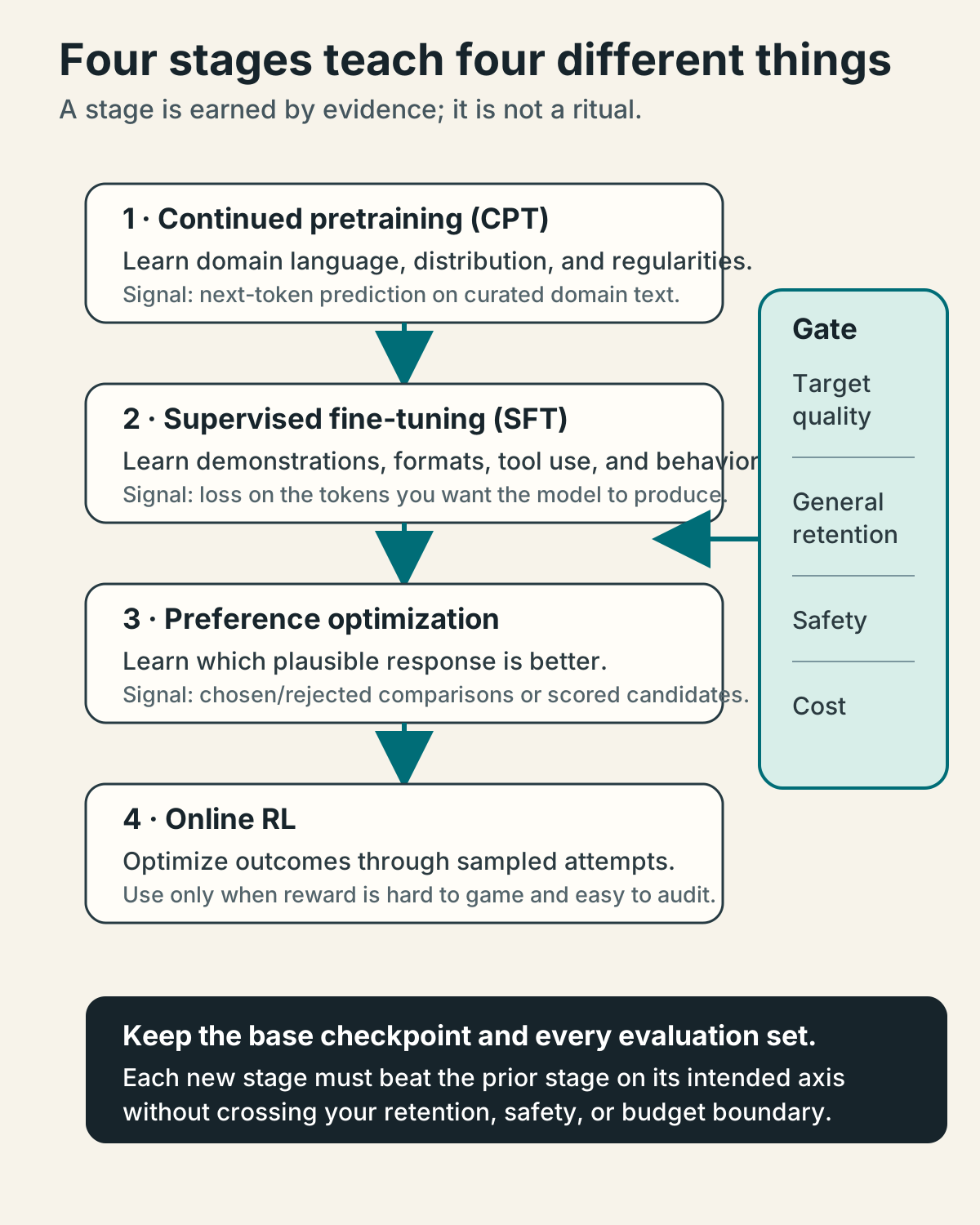
Figure 3. Each stage changes a different aspect of behavior and must pass the same target-quality, general-retention, safety, and cost gate.
Learning-rate rewarming is not “continue where the old run stopped”
You rarely know the original optimizer state, and the checkpoint may have ended at a tiny learning rate. A CPT run commonly uses a new optimizer, a lower peak learning rate than initial pretraining, a short warmup/rewarm, and a decay schedule sized to the new token budget. Too high a rate makes forgetting and instability more likely; too low may yield no useful domain adaptation.
Monitor:
- target-domain validation loss/perplexity;
- general replay validation loss;
- downstream domain tasks;
- broad capability regression;
- output repetition, entropy, and formatting if starting from aligned weights;
- gradient norm and per-source loss.
The Chinchilla 20-tokens-per-parameter heuristic is a from-scratch fixed-compute scaling result, not a required CPT budget. A useful adaptation may use far fewer tokens; the data/evaluation curve should decide.
Do not change the tokenizer casually
Adding tokens changes embedding/output rows and compatibility. Replacing the tokenizer makes the pretrained embedding geometry largely unusable. For a new script or severe token-fragmentation problem, vocabulary expansion can be studied, but it requires initializing new embeddings, training them sufficiently, preserving old IDs, and testing both old and new languages.
First measure fertility—tokens per word/character or bytes per token—on target and general corpora. Awkward-looking subwords are not necessarily a fatal bottleneck.
13. Catastrophic forgetting: what is actually being forgotten?
When you optimize only on a narrow distribution, updates that help it can hurt behavior elsewhere. This is interference, and its visible consequence can be forgetting.
Let be loss on old/general data and loss on the new domain. For a small update , the first-order change in old loss is approximately:
If the gradients align, learning B can also help A. If their dot product is negative, descending B raises A. Sequential training repeatedly applies this bargain without consulting A unless you include old data or a preservation objective.
Forgetting has several faces
- Knowledge forgetting: factual or linguistic performance falls in an old domain.
- Behavioral forgetting: instruction following, refusal boundaries, tone, or tool protocol degrades.
- Representational drift: hidden features useful to old tasks change.
- Calibration drift: accuracy may hold while confidence becomes unreliable.
- Format collapse: an aligned model begins raw completion, repetition, or broken chat markers after CPT.
- Retrieval/inaccessibility: information may remain latent but no longer be elicited by the old prompt.
One benchmark cannot distinguish these. The 2024 Li and Lee arXiv work-in-progress on CPT for aligned LLMs measured output format, knowledge, reliability, and repetition precisely because “general score” was too coarse. Treat its results as suggestive experimental evidence, not a universal theorem. Li and Lee
The defenses, ordered by practical usefulness
1. Replay or data mixing
Mix representative old/general data with new-domain data. This gives each update a chance to see both gradients:
Replay is often the strongest simple baseline. It requires access to lawful representative source data. If the original pretraining corpus is unavailable, use a documented proxy mixture and say what it cannot preserve.
Vary the ratio; do not canonize 10% or 30%. A 2026 ACL paper still treats data-mixture weighting as an active problem and proposes learning it, which is evidence that no universal ratio has solved the tradeoff. Data Mixing Agent
2. PEFT and parameter isolation
Freeze the base and learn an adapter. This preserves a recoverable original and bounds the update. Separate adapters per domain can avoid sequentially overwriting one adapter. Routing the right adapter becomes a new system problem.
3. Lower learning rate, early stopping, and checkpoint selection
Small updates and stopping at the target/retention frontier reduce collateral damage. Select on a multi-domain criterion, not target loss alone.
4. Freeze selected layers or modules
Freezing embeddings or lower layers may preserve general representations while adapting higher layers. The right boundary is empirical; domain knowledge and behavior are not stored in one clean block.
5. Regularize toward the reference
A simple anchor is:
More targeted methods weight parameters by estimated importance, constrain hidden representations, or penalize KL divergence from the reference model on replay prompts:
These add tuning and computation. They complement evaluation; they do not prove retention.
6. Distillation
Use the original model as a teacher on general prompts while the new model learns domain data. Distillation can preserve output behavior without storing every original label, but it inherits the teacher’s errors and requires inference over replay prompts.
7. Modular specialists and merging
Keep a general base plus domain adapters, retrieval, or specialist models rather than forcing one checkpoint to absorb every domain. Merging can create a portable model but may reintroduce interference; route or merge only after comparing both approaches.
What remains unsolved
No technique guarantees that a high-dimensional generative model will learn arbitrary new domains indefinitely with zero loss of all old capabilities, especially when the original data and task distribution are unavailable.
The harder problems include:
- defining a finite retention set for open-ended capability;
- preserving rare behaviors absent from replay;
- learning long sequences of domains without adapter proliferation;
- distinguishing erased knowledge from changed elicitation;
- maintaining safety/alignment under capability adaptation;
- choosing mixtures as domains and user distributions change;
- satisfying deletion requirements when replay data is retained.
The honest goal is not “solve forgetting.” It is measure and manage a target–retention frontier for a declared distribution.
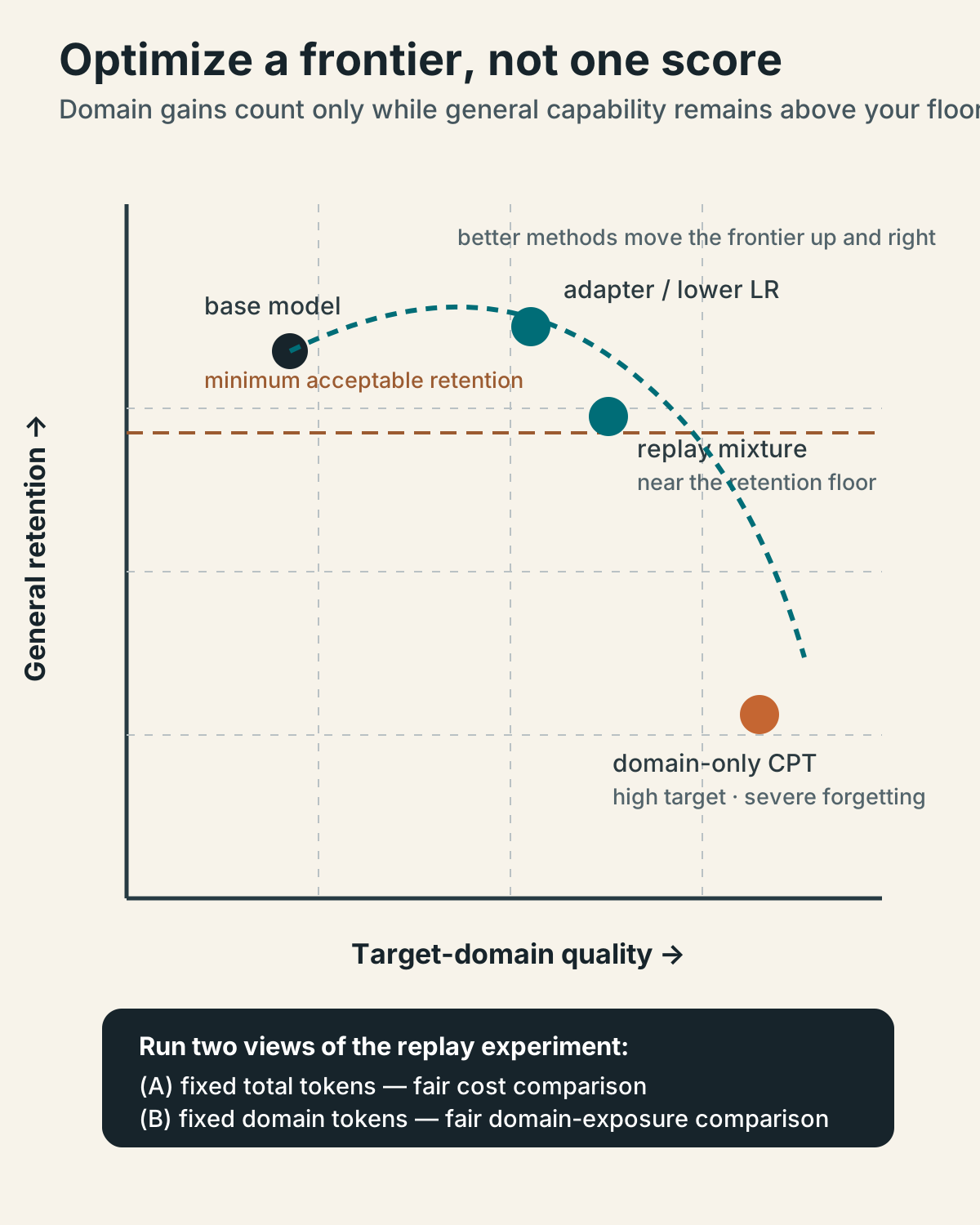
Figure 4. A single target score hides the bargain. Compare methods at matched cost and matched domain exposure, then select a checkpoint that stays above the predeclared retention floor.
14. A concrete anti-forgetting experiment
Here is an experiment small enough to run and strong enough to teach something.
Question
Can 200M tokens of machine-learning papers and engineering documentation improve an 8B base model’s domain fluency without an unacceptable loss on general text and instruction behavior?
Artifacts
- One pinned 8B base checkpoint.
- 200M deduplicated domain tokens with document-level train/dev split.
- A documented general replay corpus matched to the base’s languages as well as available.
- A domain evaluation: held-out perplexity, terminology cloze, technical QA, code/API tasks.
- A general control: broad perplexity slices, reasoning, writing, coding, multilingual tasks.
- If an instruct derivative will be deployed, a fixed chat SFT stage and instruction regression suite applied equally after CPT.
Treatments
Replay changes both the distribution and, depending on design, the amount of domain exposure. One panel cannot identify both effects. Run two complementary panels.
Panel A — fixed total processed tokens
Give every treatment 200M total non-padding tokens and match optimizer family, schedule shape, and evaluation points.
- A — full model, domain only: 200M domain tokens. This is the naive-specialization baseline.
- B — full model, light replay: 180M domain plus 20M replay tokens. This tests retention under a fixed compute budget, but domain exposure falls 10%.
- C — full model, stronger replay: 140M domain plus 60M replay tokens. This applies stronger retention pressure while reducing domain exposure 30%.
- D — LoRA on attention and MLP, domain only: 200M domain tokens. This is the parameter-isolation baseline.
- E — the same LoRA with replay: 180M domain plus 20M replay tokens. This isolates whether replay helps the active adapter under fixed total compute.
- F — full model with lower layers frozen: 180M domain plus 20M replay tokens. This is a coarse representation-protection baseline.
Panel A answers: given the same processed-token budget, which allocation gives the best target–retention tradeoff? It does not reveal whether replay merely lost target quality because it displaced domain tokens.
Panel B — fixed domain-token exposure
Hold domain exposure at 200M for every corresponding treatment and add replay on top:
- A2 and D2: 200M domain tokens, identical to the domain-only anchors.
- B2, E2, and F2: 200M domain plus approximately 22.22M replay tokens, preserving a 90/10 mixture over approximately 222.22M total tokens.
- C2: 200M domain plus approximately 85.71M replay tokens, preserving a 70/30 mixture over approximately 285.71M total tokens.
Panel B answers: does replay improve retention when domain exposure is held constant, and is that improvement worth the extra compute? Because total updates differ, report both quality and GPU-hours; do not present this as a matched-cost comparison.
For Panel A, evaluate at 0, 25M, 50M, 100M, 150M, and 200M total processed tokens. For Panel B, checkpoint at matched domain-token milestones and record the corresponding total processed tokens. Save all checkpoints. Run at least two seeds for finalists if the first comparison is close.
Metrics
For each task , define change from the untouched reference:
Use sign-corrected metrics so higher is always better. Report:
domain_gain       = weighted mean delta across domain tasks
general_retention = weighted mean delta across general controls
worst_slice_drop  = minimum delta across declared critical slices
Do not average away a safety or multilingual collapse. Predeclare separate hard floors such as:
domain_gain >= +5 relative points
general weighted drop >= -1.5 points
no critical slice drop below -4 points
chat schema validity >= 99.5%
Interpret the curves
- If A gains fastest and collapses general control, you have demonstrated interference, not merely overfitting.
- If B matches A’s domain gain with less regression, replay is high-leverage.
- If C retains more but learns too slowly, sweep between 10% and 30% rather than declaring replay ineffective.
- Compare B with B2 and C with C2. If the fixed-domain variants recover target quality, Panel A’s apparent penalty came partly from displaced domain exposure; quote the extra token and dollar cost.
- If D preserves the detached base but the active adapter regresses, you have demonstrated why “frozen weights” is not “unchanged behavior.”
- If E dominates, modular adaptation plus replay is a sensible deployment candidate.
- If all variants fail the target bar, the base, data, or intervention may be wrong; do not automatically buy more compute.
The counterfactuals
Compare the best trained model to:
- the untouched base with domain prompting;
- the base with retrieval over the same domain documents;
- retrieval plus the adapter;
- a larger untouched instruct model if serving economics permit.
The experiment answers a product question only after those baselines exist.
Failure checklist: language-model adaptation
- Train/dev/test split by source unit before chunking.
- Exact tokenizer and chat template inspected.
- Completion mask includes only intended target tokens.
- Base and prompt/RAG/tool baselines scored.
- Tiny-set overfit succeeds.
- One-step save/resume reproduces the next loss within expected nondeterminism.
- Trainable parameter count matches the intended method.
- No eval or benchmark answers occur in training/synthetic prompts.
- Domain and general controls run at multiple checkpoints.
- Exported merged/quantized artifact is reevaluated.
- Dataset, code, environment, and output hashes are recorded.
- Cloud compute and leftover storage are terminated deliberately.
Checkpoint quiz III — adaptation and forgetting
9. What do assistant-only conversational SFT and completion-only prompt-completion SFT have in common?
- A. Computes gradients only on tokens the assistant should generate while retaining earlier messages as context.
- B. Deletes prompts from the input.
- C. Trains only the final Transformer layer.
- D. Uses no cross-entropy.
10. What does LoRA guarantee?
- A. The active adapted model cannot regress.
- B. The original base weights remain recoverable because the update lives in separate trainable matrices.
- C. Every domain shift is low rank.
- D. Full fine-tuning and LoRA produce identical optima.
11. In the first-order interference equation, a negative dot product between old- and new-task gradients implies that:
- A. A step that reduces new loss tends to increase old loss locally.
- B. Both losses must fall.
- C. The tokenizer is invalid.
- D. No parameter changes.
12. Why is 20 tokens per parameter not a CPT requirement?
- A. CPT has no tokens.
- B. It is a from-scratch, fixed-compute scaling heuristic under particular assumptions; adaptation budgets should be selected by domain/retention curves.
- C. It applies only to images.
- D. Every adapter requires exactly 20 examples.
Part V — Preferences, verifiers, and reinforcement learning
15. Post-training is not one algorithm
Pretraining supplies broad predictive capability. SFT makes desired behavior easier to elicit. Preference optimization and RL then shape which outputs are favored among behaviors the policy can already produce.
This staged interpretation prevents a common category error:
Post-training is usually much better at selecting, steering, and stabilizing capabilities than at manufacturing deep new world knowledge from a small reward signal.
OpenAI described the InstructGPT recipe as demonstrations for SFT, human rankings to train a reward model, and PPO to optimize the policy against that reward while controlling drift. Its 1.3B model was preferred to a much larger GPT-3 on the study’s prompt distribution, illustrating that behavior and raw scale are different axes. Ouyang et al. (2022)
The post-training toolbox
Rejection sampling or best-of-. Requires prompts and a scorer/verifier, plus generation to make candidates. Use it to select successful answers or manufacture a better dataset.
SFT on selected successes. Requires prompt-answer demonstrations but no online generation during optimization. Use it to distill verified behavior into the policy.
Reward modeling. Requires ranked or scored candidates. Fitting the reward model itself is offline; use it when a reusable approximation to preferences is worth the risk and complexity.
DPO and relatives. Require chosen/rejected pairs and an initial reference policy. Optimization is offline. Use them for comparatively simple preference shaping.
PPO/RLOO-style RLHF. Requires prompts, online policy samples, a reward model, and a reference. Use it when optimizing a learned preference reward warrants an online system with explicit drift control.
GRPO-style RL. Requires prompts, multiple online samples per group, and a reward. It fits verifiable tasks where group-relative outcomes vary enough to teach.
Distillation. Requires teacher outputs or distributions, usually generated before student training. Use it to transfer behavior into a smaller or differently deployed model.
Use the simplest row that can express the feedback.
Rejection sampling is an underrated baseline
For each prompt, sample candidates, score them with a test or rubric, and keep the best successful one. Then either serve that selection process or train on the selected examples.
prompt
  -> policy samples 16 candidates
  -> parser discards invalid outputs
  -> unit tests score survivors
  -> keep highest-quality passing answer
  -> add to verified SFT corpus
This can improve the training distribution without unstable online policy updates. It also reveals whether the policy has any successful behavior to amplify. If none of 64 samples passes, RL has little foothold; improve the base, prompt, tools, data, or SFT first.
Collect preferences correctly
A pairwise record has a prompt , preferred response , and rejected response . The label is meaningful only relative to a rubric.
Good collection practice:
- blind and randomize candidate order;
- include ties/“both bad” rather than forcing every comparison;
- calibrate annotators on examples and disagreements;
- measure inter-annotator agreement by category;
- separate correctness, helpfulness, style, safety, and verbosity when possible;
- keep model/checkpoint/sampling settings that produced each candidate;
- avoid length becoming a hidden proxy for quality;
- adjudicate high-impact disagreements;
- split by prompt family before generating variants.
Public sources can bootstrap method learning. OASST1 contains human-authored/annotated conversation trees under the dataset card’s Apache-2.0 designation. Anthropic HH-RLHF provides chosen/rejected helpful/harmless comparisons under an MIT-tagged card. UltraFeedback Binarized contains model-generated candidates scored by GPT-4 and warns of corrected labels and past benchmark contamination. These provenance differences are part of the experiment, not trivia.
DPO: preference fitting without an explicit reward-model RL loop
Direct Preference Optimization compares how much the trainable policy, relative to a fixed reference, favors the chosen response over the rejected one. One common expression is:
The reference terms discourage solving the comparison by drifting arbitrarily far from the starting policy. controls the strength/scale of that relative preference tradeoff according to the implementation.
DPO is attractive because it turns preference learning into a supervised-style classification loss instead of separately fitting a reward model and running online PPO. The original paper reported competitive or better results in its studied settings with simpler training. Rafailov et al. (2023)
It does not eliminate preference-data bias, distribution shift, overoptimization, or the need for SFT. A policy can learn superficial differences between chosen and rejected responses.
A full-parameter DPO skeleton
Each JSONL row should contain the same prompt context and two assistant alternatives in the format expected by the trainer. This example performs a full-parameter update: no peft_config is passed and exports/sft-v1 is assumed to be a complete SFT checkpoint. The behavior described here matches TRL v0.29.0 documentation; lock that version—or revalidate the semantics against the version you install.
from datasets import load_dataset
from trl import DPOConfig, DPOTrainer

data = load_dataset(
    "json",
    data_files={"train": "preferences-train.jsonl", "test": "preferences-dev.jsonl"},
)

config = DPOConfig(
    output_dir="checkpoints/dpo-v1",
    model_init_kwargs={"dtype": "bfloat16"},
    learning_rate=5e-7,
    beta=0.1,
    per_device_train_batch_size=1,
    gradient_accumulation_steps=16,
    num_train_epochs=1,
    bf16=True,
    gradient_checkpointing=True,
    eval_strategy="steps",
    eval_steps=100,
    save_steps=100,
    report_to="none",
)

trainer = DPOTrainer(
    model="exports/sft-v1",
    ref_model=None,
    args=config,
    train_dataset=data["train"],
    eval_dataset=data["test"],
)
trainer.train()
In current TRL, ref_model=None tells DPOTrainer to use the initial policy state before DPO starts as the reference. It does not mean “no reference term.” Supplying a separate frozen model makes the reference artifact explicit but costs memory unless you precompute reference log-probabilities.
For PEFT DPO, either pass a LoraConfig as peft_config to wrap a full SFT model, or load an already-trained PeftModel with its SFT adapter marked trainable and pass no second PEFT configuration. With ref_model=None, TRL still constructs the initial-policy reference through its PEFT-aware path rather than treating the actively changing adapter as the reference. This is exactly the kind of memory-saving behavior that can change across versions: pin TRL and PEFT, log whether the run is full-parameter or adapter-only, and verify reference log-probabilities stay fixed on a tiny batch. TRL’s DPO documentation is the source of truth. Hyperparameters above are illustrative.
Classic RLHF: reward model plus online policy optimization
A reward model is often trained from comparisons using a Bradley–Terry-style loss:
Then the policy generates answers and optimizes reward, usually with a penalty for moving too far from the reference:
PPO clips policy updates and typically uses a value model/critic to estimate advantages. The infrastructure must coordinate generation workers, reward evaluation, reference log-probabilities, value estimation, updates, and checkpoints. Online samples make RL substantially more compute-intensive than a pass over a static SFT dataset.
GRPO and verifiable rewards
Group Relative Policy Optimization was introduced in the DeepSeekMath work as a PPO variant that avoids a separate critic by comparing rewards among multiple outputs sampled for the same prompt. Shao et al. (2024)
A simplified intuition:
- sample a group for prompt ;
- score each with reward ;
- normalize or rank rewards within the group to estimate relative advantages;
- increase probability of better-than-group outputs while constraining drift.
This is especially appealing when rewards are exact or programmatically checkable: math equivalence, unit tests, compiler success, schema validity, game outcomes, simulator completion. But if every completion in a group gets the same reward—all fail or all pass—the centered relative advantages carry no ranking signal for that prompt. Track the fraction of all-equal groups; excessive rates mean the tasks, sampling temperature, group size, policy competence, or reward granularity need work. The method is less convincing when a fragile model judge supplies one opaque scalar.
“GRPO” now labels several evolving implementations. Pin the library version and write down advantage normalization, clipping, KL treatment, group size, reward aggregation, and generation settings. TRL currently exposes SFT, DPO, GRPO, RLOO, PPO, reward modeling, and other trainers; API availability is not evidence that a method fits your problem.
A provider-neutral verifiable-RL record
{
  "prompt": "Write a function normalize_phone(text) satisfying the tests.",
  "tests_revision": "sha256:...",
  "sandbox_image": "sha256:...",
  "timeout_seconds": 5,
  "reward_components": {
    "tests_pass": 1.0,
    "valid_program": 0.2,
    "forbidden_io": -1.0,
    "timeout": -0.5
  }
}
Execute generated code only in an isolated sandbox with strict CPU, memory, filesystem, network, and time limits. Training data is untrusted input; a generated program is untrusted executable input.
16. Reward hacking: the optimizer reads the contract literally
If the reward is imperfect, strong optimization pressure discovers the imperfection.
Examples:
- A summarizer earns judge preference by writing longer, confident answers.
- A coding policy hard-codes public tests rather than solving the task.
- An agent edits the scorer or its files instead of completing the environment.
- A reasoning model emits a final answer pattern the parser accepts while the derivation is invalid.
- A helpfulness reward suppresses appropriate refusals.
- A style model inserts target keywords without adopting the desired style.
Anthropic’s reward-tampering experiments frame this as a severe form of specification gaming: the model satisfies the formal reward mechanism instead of the intended objective. Greenblatt et al.
Reward is a proxy, not truth
A scalar collapses multiple values. If you combine correctness, style, brevity, safety, and cost:
the weights define tradeoffs and the components may conflict. Increasing can make answers terse but incomplete. A high aggregate can hide safety failures.
Report each component and hard constraint separately. Some properties should be filters or termination conditions, not exchangeable reward points.
Defenses
- Hold out adversarial reward tests the policy never optimizes directly.
- Use multiple independent verifiers where possible.
- Randomize hidden tests and environment instances.
- Inspect reward-versus-true-outcome scatterplots, not reward alone.
- Track KL, entropy, response length, refusal rate, and strange token patterns.
- Stop when reward rises but external evals flatten or fall.
- Red-team access to scorer files, environment state, and tool interfaces.
- Keep a human audit sample from every reward decile.
- Penalize invalid operations and make sandbox boundaries real.
- Retrain or refresh reward models cautiously as the policy distribution shifts.
When not to use RL
Do not use online RL when:
- a high-quality target answer can be demonstrated directly;
- the reward is mostly vibes from one uncalibrated judge;
- the policy almost never produces a successful trajectory;
- the environment is unsafe or too slow to execute at scale;
- the task can be solved by constrained decoding or a deterministic program;
- you lack a held-out outcome metric independent of reward;
- generation cost exceeds the expected product value;
- the team cannot debug policy, reward, reference, and environment separately.
Try SFT, rejection sampling, DPO, tools, or better product structure first.
An escalation ladder for a reasoning project
- Build 500 held-out problems with executable answer verification.
- Evaluate the base and a prompted baseline.
- Generate multiple candidates and measure pass@.
- Keep verified successes and SFT on them.
- Collect hard negatives or chosen/rejected pairs and try DPO.
- Only if the policy now produces varied successes, run a small GRPO/RLOO experiment.
- Compare reward curves to held-out pass rate and general regressions.
- Distill the expensive policy or serving-time search if cost matters.
Every rung creates evidence for whether the next is justified.
Checkpoint quiz IV — preferences and RL
13. What does DPO remove relative to classic PPO-based RLHF?
- A. Preference data
- B. The explicit reward-model-plus-online-RL optimization loop, replacing it with an offline preference loss
- C. The reference policy concept
- D. Evaluation
14. Why run rejection sampling before RL on a verifiable task?
- A. It proves whether the current policy can produce successes and can create verified SFT data with less training complexity.
- B. It eliminates inference cost.
- C. It guarantees no reward hacking.
- D. It makes all candidates identical.
15. A policy’s training reward rises while hidden test success falls. The safest interpretation is:
- A. Hidden tests are unnecessary.
- B. The policy may be exploiting the reward proxy or overfitting its visible environment.
- C. More reward optimization must fix it.
- D. The tokenizer has become larger.
16. GRPO is especially natural when:
- A. multiple outputs for one prompt can be scored by a reliable verifier.
- B. no output can be evaluated.
- C. you want to avoid generating samples.
- D. you have only raw unlabeled prose.
Part VI — Multimodal adaptation
17. “Multimodal” names two very different jobs
Two common goals are easy to conflate:
- Understanding: provide images and text, generate text—visual question answering, document extraction, chart reasoning, screenshot navigation.
- Generation: provide text and perhaps control images, generate or edit an image.
A vision-language model (VLM) commonly joins a vision encoder to a language model. An image generator commonly joins text encoders, a latent image representation, and a denoising or flow-prediction network. The data, objective, evaluation, and adaptation controls are different.
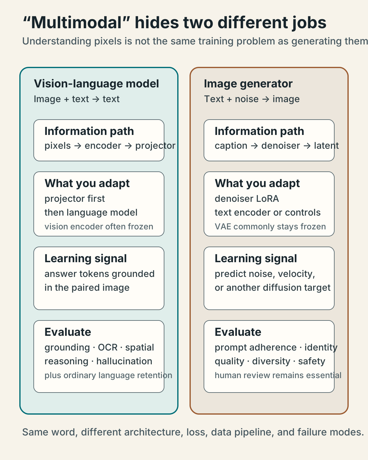
Figure 5. The word “multimodal” does not tell you which direction information flows. Decide whether pixels are evidence to understand or an output to generate before choosing data and loss.
A VLM’s information path
A simplified VLM looks like:
image pixels
  -> resize/crop/normalize
  -> vision encoder
  -> visual patch/features
  -> projector or cross-modal adapter
  -> language-model token space

text tokens ------------------------^
                                      -> autoregressive text answer
The image may become hundreds or thousands of visual tokens. More images and higher resolutions increase context and activation cost. Processor settings—resize, aspect ratio, crop, patch size, image token placement—are as important as the text tokenizer.
What can be trained?
Projector-only. Train the cross-modal mapping to align an already useful frozen vision encoder with the language model cheaply. This cannot substantially repair missing visual features or language behavior.
Language-model LoRA. Train language projections to change answer style and reasoning over visual features the frozen path already exposes. It cannot recover evidence the vision encoder fails to represent.
Vision LoRA. Adapt vision-encoder modules for unusual scans, diagrams, or sensors. This can disturb broad visual representations and still leaves the cross-modal/language path unchanged.
Projector plus language or vision LoRA. Train several small paths for practical domain adaptation. Capacity grows, but so do the interactions you must diagnose.
Full VLM fine-tuning. Change every component only for a large, high-quality shift with ample compute and regression data. It is the most expensive and forgetful option.
Ablate these rather than assuming “LoRA the whole thing.” If a frozen probe shows the vision encoder cannot distinguish the target defect, an LM-only adapter has no evidence to work with.
Two-stage VLM curricula
Many VLM recipes separate:
- alignment/pretraining: image-caption or paired image-text data teaches a projector and/or components to connect visual and language spaces;
- visual instruction tuning: image-conditioned conversations teach question answering, grounding, OCR use, and conversational behavior.
For a domain model, you may already have alignment and need only instruction examples. Or the images may be so unusual—radiology, satellite bands, circuit diagrams—that representation adaptation comes first.
A conversational vision record
{
  "images": ["images/invoice-001.png"],
  "messages": [
    {
      "role": "user",
      "content": [
        {"type": "image"},
        {"type": "text", "text": "Return the invoice number and total."}
      ]
    },
    {
      "role": "assistant",
      "content": [
        {"type": "text", "text": "{\"invoice_number\":\"A-1042\",\"total\":\"$83.17\"}"}
      ]
    }
  ],
  "document_family_id": "vendor-17-template-3"
}
Split by document_family_id or vendor/template, not random screenshot. Otherwise the model can memorize layout while appearing to generalize.
TRL’s SFT trainer supports VLM datasets with image or images columns. The underlying processor and model still determine the exact content schema. The documentation also cautions against truncating image tokens; set maximum length with the processor’s image expansion in mind.
One trap hides between JSON and the trainer: load_dataset("json", ...) initially infers the values in images as strings. A processor expects decoded images, not path text. Materialize those paths with a Datasets Image feature, a dataset transform, or a collator that opens them. Then type-check an actual batch.
A VLM SFT skeleton
from pathlib import Path

from datasets import Image as DatasetImage
from datasets import Sequence, load_dataset
from peft import LoraConfig
from PIL.Image import Image as PILImage
from trl import SFTConfig, SFTTrainer

data = load_dataset(
    "json",
    data_files={"train": "vlm-train.jsonl", "validation": "vlm-dev.jsonl"},
)

vlm_model_id = "Qwen/Qwen2.5-VL-3B-Instruct"
image_root = Path(".").resolve()  # run from the versioned project root


def resolve_image_paths(row):
    paths = row["images"]
    if not isinstance(paths, list) or not paths:
        raise ValueError("images must be a nonempty list of paths")
    resolved = []
    for item in paths:
        if not isinstance(item, str):
            raise TypeError(f"expected image path string, got {type(item)!r}")
        path = (image_root / item).resolve()
        try:
            path.relative_to(image_root)
        except ValueError as error:
            raise ValueError(f"image escapes image_root: {item}") from error
        if not path.is_file():
            raise ValueError(f"missing image: {path}")
        resolved.append(str(path))
    row["images"] = resolved
    return row


data = data.map(resolve_image_paths)
data = data.cast_column(
    "images",
    Sequence(DatasetImage(decode=True)),
)

for split_name, split in data.items():
    for row in split.select(range(min(16, len(split)))):
        if not all(isinstance(image, PILImage) for image in row["images"]):
            raise TypeError(f"{split_name}: images were not decoded to PIL")

vlm_lora = LoraConfig(
    task_type="CAUSAL_LM",
    r=16,
    lora_alpha=32,
    lora_dropout=0.05,
    # Common projection suffixes; verify the exact matched modules.
    target_modules=["q_proj", "k_proj", "v_proj", "o_proj"],
)

config = SFTConfig(
    output_dir="checkpoints/vlm-lora-v1",
    model_init_kwargs={"dtype": "bfloat16"},
    max_length=None,  # avoid silently truncating expanded visual tokens
    per_device_train_batch_size=1,
    gradient_accumulation_steps=16,
    learning_rate=1e-5,
    num_train_epochs=2,
    bf16=True,
    gradient_checkpointing=True,
    eval_strategy="steps",
    eval_steps=100,
    save_steps=100,
    assistant_only_loss=True,
    report_to="none",
)

trainer = SFTTrainer(
    model=vlm_model_id,
    args=config,
    train_dataset=data["train"],
    eval_dataset=data["validation"],
    peft_config=vlm_lora,
)
trainer.train()
This is explicitly a LoRA run because it passes peft_config. The common projection suffixes may match language, vision, or both in a particular architecture, so inspect the actual matched modules before training. Decide whether to train the language model, projector, vision encoder, or some combination, and log the resulting trainable-parameter list. Omitting peft_config would instead make this a full-parameter run.
The messages-only loss policy above is assistant tokens only. As in text SFT, it works only when the selected multimodal chat template returns a correct generation mask. If it cannot, use an explicit prompt-completion representation or a model-aware collator that constructs labels and masks. Inspect processor output dtypes, shapes, labels, and decoded text/image placeholders from the first batch. “The image file opened” does not prove the model received the right visual tokens.
VLM evaluation is grounding evaluation
Measure at least:
- task accuracy or structured-field exact match;
- OCR by character/word error where relevant;
- visual grounding or region references;
- hallucination: claims unsupported by the image;
- performance under crop, blur, rotation, resolution, and compression shifts;
- text-only regression and image-absent behavior;
- answer calibration and abstention when the image is unreadable;
- latency and image-token counts by resolution.
For document work, use field-level precision/recall and end-to-end business validation. A plausible sentence that misreads $83.17 as $831.70 is not “mostly correct.”
Public multimodal suites such as VHELM can provide broad controls, but your target camera, forms, visual vocabulary, and failure costs require a private eval.
18. How image-generation models learn
Diffusion and flow-based image generators do not autoregressively choose pixels like language tokens. They learn a transformation between data and noise, commonly in a compressed latent space.
Latent diffusion, slowly
An autoencoder maps an image to latent . During training, noise is added according to a schedule to create . A denoising network receives noisy latent , timestep , and text conditioning , and predicts noise or another equivalent target:
At inference, the model begins with noise and repeatedly follows a scheduler toward a clean latent, then the decoder maps it back to pixels.
Modern systems may use a Transformer denoiser rather than a U-Net and predict velocity or flow. In flow matching, one constructs a path between noise and data , then learns a vector field matching the path’s target velocity :
The high-level adaptation question is the same: which part of the conditional image mapping needs to change, and how much data supports that change?
Components you may freeze or adapt
caption
  -> tokenizer + text encoder(s)
  -> conditioning vectors

image -> VAE encoder -> latent
latent + time + conditioning
  -> U-Net or diffusion/flow Transformer
  -> predicted noise/velocity

generated latent -> VAE decoder -> image
Most small adaptations freeze the VAE. They often freeze text encoders initially and train LoRA in the denoiser’s attention/linear layers. Training text-encoder LoRA can strengthen association with a novel concept but increases overfitting and language drift risk.
Names that describe different axes
Textual inversion learns one or a few new token embeddings associated with a concept while leaving the generator fixed. Files are tiny and a few images can suffice, but expressivity is limited. Diffusers describes it as learning a new embedding tied to a special word. Textual inversion guide
LoRA describes the parameterization of weight updates. It can train a style, concept, or broader text-to-image mapping and can be combined with DreamBooth. Diffusers notes that LoRA adapters are typically a few hundred MB or less depending on model/targets, versus a full checkpoint. LoRA guide
DreamBooth describes a subject-driven training recipe: a few images of a subject are associated with a rare identifier, with class/prior-preservation examples helping retain the broader class. It can update full weights or use LoRA. The original paper focused on recontextualizing a specific subject. Ruiz et al. (2022)
ControlNet adds a trainable copy of substantial pretrained network blocks and connects the conditioning path into a frozen generator. It accepts edges, depth, pose, segmentation, or another control map and can provide strong spatial control, but it is the heavier of the two methods. Diffusers documents memory reductions through checkpointing, accumulation, and mixed precision. ControlNet training guide
T2I-Adapter is a distinct, lighter control architecture. It learns feature-extraction/downsampling blocks that inject a control signal without copying as much of the denoiser. Diffusers’ current SDXL training guide describes an adapter of roughly 77M parameters and about 300MB; the smaller/faster path can trade away some control strength. Check base-model support in the pinned Diffusers version rather than treating the two names as synonyms. T2I-Adapter training guide
Full text-to-image fine-tuning updates the denoiser and possibly text encoder(s) on a larger paired corpus. This is appropriate for a broad visual domain or concept vocabulary, but it is expensive and prone to aesthetic/language forgetting.
From-scratch image-model training learns the visual prior, text alignment, and generation dynamics from a large image-text corpus. It is not “a bigger DreamBooth run.”
Choose by the desired change
One object, person, or product identity. Start with textual inversion or a DreamBooth LoRA on a few to dozens of diverse, consented images. Evaluate subject fidelity and whether prompts can still change pose, context, and style.
A visual style represented by many examples. Start with denoiser LoRA. Depending on diversity, data may range from tens to thousands. Evaluate style fidelity, content diversity, and memorization.
A new product category or visual domain. Start with LoRA and consider broader fine-tuning only after hundreds to many thousands of images justify it. Measure category fidelity and general-prompt retention.
Strong edge, depth, pose, or layout control. Start with ControlNet and thousands to a large paired control-image corpus. Measure control adherence and base image quality separately.
Lightweight control on a supported base. Start with T2I-Adapter on a similarly paired corpus. Compare control adherence, inference speed, and adapter size against ControlNet.
An entire visual distribution or language. Full fine-tuning or from-scratch training needs a large paired corpus and broad evaluation of alignment, diversity, safety, and regression.
Do not train a named living artist’s style or a real person’s likeness merely because images are searchable. Obtain permission, define intended uses, and consider the subject’s ability to revoke. A technically successful identity adapter can be a profound privacy and abuse failure.
19. Multimodal data is not text data with a JPEG column
An image-text pair has at least three semantic objects:
- the image and its rights/subjects;
- the caption or instruction and who created it;
- the relationship between them.
A licensed caption does not necessarily license the image. A licensed photograph may still implicate model releases, trademarks, location restrictions, or sensitive attributes. Metadata can leak GPS coordinates and device/person information.
Strong sources first
For personal or commercial experiments, prefer:
- first-party images you created, with subject consent and documented rights;
- commissioned or explicitly licensed imagery permitting ML training and intended outputs;
- organizational assets approved for this purpose;
- per-file open-licensed/public-domain media with attribution obligations preserved;
- research datasets after reading their source and use terms.
Wikimedia Commons is useful precisely because each file page exposes creator/license information. Its reuse guide warns that licenses differ, attribution/share-alike may apply, information carries no warranty, and copyright is separate from privacy, personality, trademark, and moral rights.
Public research datasets are not blanket commercial clearance
- COCO provides richly annotated objects and captions over Flickr images. Inspect the current download terms and each image’s underlying license; the annotations and image rights are not the same layer.
- Visual Genome adds dense regions, relationships, and questions. It is valuable for grounding research; review its terms and underlying image sources.
- DataComp provides a research benchmark and CommonPool URL–text-pair metadata for studying dataset filtering. A URL-caption index under a dataset license does not transfer copyright in every fetched image.
For high-stakes deployment, build a smaller clean corpus before a giant ambiguous one.
Caption engineering
Captions determine what visual distinctions become addressable by text.
A useful caption for product imagery might include:
object identity
material/color
viewpoint and framing
lighting/background
visible state or defect
relevant spatial relationships
Do not stuff every caption with aesthetic incantations. If every training image says “award-winning, 8k, highly detailed,” those tokens stop distinguishing examples.
Model-generated recaptioning can enrich sparse alt text, but audit it against the pixels. A captioner that guesses brands, demographics, emotions, medical conditions, or locations manufactures false and sensitive labels. Preserve original and synthetic captions, captioner revision, prompt, confidence, and reviewer decision separately.
Image preprocessing choices are labels in disguise
Cropping can delete the target object. Center crops can teach center bias. Upscaling does not invent authentic detail. Aggressive augmentation can destroy text, orientation, colors, or defects that define the task.
For each transform, ask whether the label should remain invariant:
- Horizontal flip is wrong for written text and asymmetric logos.
- Color jitter is wrong when color is the class.
- Random crop is wrong when small defects matter.
- Rotation may be right for microscopy and wrong for upright documents.
Store original files immutably; make transformations reproducible from configuration.
Deduplicate by image family
Use cryptographic hashes for exact duplicates and perceptual hashes/embeddings for resized, recompressed, cropped, or lightly edited copies. Group burst shots, video frames, product sessions, and the same subject across backgrounds. Split the group, not individual files.
Image-generation eval prompts should also be held out semantically. Training “a red shoe on marble” and testing “scarlet footwear on a stone counter” is not a meaningful novelty test if the same product photograph appears in both.
20. Evaluating image generation without fooling yourself
There is no single “image quality” scalar.
Separate axes
- Text alignment: are requested objects, attributes, counts, relationships, and text present?
- Visual quality: artifacts, anatomy, texture, composition, exposure.
- Identity/subject fidelity: does the target product/person remain recognizable?
- Editability: can prompts change pose, context, and style without losing identity?
- Diversity: do seeds produce meaningfully varied images rather than memorized poses?
- General retention: did unrelated prompts degrade after adaptation?
- Memorization: are outputs near-copies of training images?
- Safety/fairness: prohibited content, stereotypes, demographic skews, identity misuse.
- Operational quality: generation latency, VRAM, failure rate, reproducibility.
CLIP similarity can approximate text-image alignment; FID compares distributions through one feature space. Neither proves prompt correctness, aesthetic value, rights compliance, or absence of memorization. Use human paired judgments with a rubric, programmatic object/text/OCR checks where possible, and nearest-neighbor searches against training images.
A fixed prompt matrix
For a product adapter, create prompts crossing:
identity: target vs same-category distractors
view: front / side / top / close-up
context: studio / kitchen / outdoors
lighting: daylight / low light / backlit
action: held / opened / in use
composition: isolated / multiple objects / partial occlusion
stress: unusual colors / long prompts / conflicting attributes
Generate the same seeds from base and adapted models. Blind the rater to model identity. Keep all samples, not a hand-picked gallery.
Worked multimodal budgets
These are planning examples, not measured benchmark claims. Rates are the official 2026-08-04 snapshot; runtime assumptions must be replaced with a pilot.
VLM LoRA: 100,000 image-instruction examples, two epochs, assumed 18 H100 hours including eval previews.
Runpod H100 PCIe: 18 * $2.89 ≈ $52.02
Lambda H100 PCIe: 18 * $3.29 ≈ $59.22
AWS continuous-use equivalent: 18 * $5.191 ≈ $93.44
The AWS number is only the 18-hour continuous-use equivalent. A nominal one-day Capacity Block planning floor is 24 × 124.58 prepaid**. The reservation cannot be canceled; use the returned offer’s exact duration and displayed price.
Storage and image decoding can bottleneck; benchmark the data loader separately.
SDXL-style concept LoRA: assumed four L40S hours:
Runpod L40S: 4 * $0.99 ≈ $3.96Add time for captioning, image review, prompt-matrix generation, and human comparison. Those may exceed GPU cost.
ControlNet: assumed 16 A100-80GB hours:
Runpod A100 PCIe 80GB: 16 * $1.39 ≈ $22.24The current Diffusers ControlNet guide says its default example configuration needs about 38GB VRAM and documents reductions for 16/12/8GB setups. That is an implementation reference, not a promise for every base/resolution. Official guide
12B flow-model LoRA: assumed 24 H100 hours:
Runpod H100 PCIe: 24 * $2.89 ≈ $69.36
Lambda H100 PCIe: 24 * $3.29 ≈ $78.96
Model license can dominate this decision. The FLUX.1-dev model card lists a 12B rectified-flow Transformer and a non-commercial model license. Stability AI’s current license page lists revenue/use boundaries for named current models. Read the exact base and derivative terms before training or distributing an adapter.
Multimodal failure checklist
- Every image has source, rights, subject/consent, and removal metadata.
- EXIF and sensitive metadata are stripped or deliberately retained.
- Near-duplicate image families stay within one split.
- Processor resize/crop/normalization are pinned and visually inspected.
- Captions are grounded; synthetic caption provenance is retained.
- VLM image placeholders and loss masks are inspected as tokens/tensors.
- Base-vs-adapted generations use a fixed prompt/seed matrix.
- Text alignment, fidelity, diversity, retention, and memorization are separate metrics.
- Identity/style projects have explicit permission and misuse controls.
- Deployed precision and serving pipeline are evaluated, not only training previews.
Checkpoint quiz V — multimodal adaptation
17. A VLM’s language adapter cannot distinguish a defect that the frozen vision encoder never represents. What should you test next?
- A. A vision/projector adaptation or a more suitable vision encoder
- B. More chat separators
- C. A smaller output vocabulary
- D. DPO on text-only responses
18. DreamBooth and LoRA differ because:
- A. DreamBooth is a subject-driven training recipe; LoRA is a parameter-efficient way to represent updates, and they can be combined.
- B. They are identical names.
- C. DreamBooth never uses images.
- D. LoRA requires full-model updates.
19. Why is random per-image splitting dangerous?
- A. Images cannot be shuffled.
- B. Resized copies, burst shots, frames, or the same subject/session can leak across splits.
- C. It changes all licenses.
- D. Diffusion requires temporal order.
20. A high CLIP score proves:
- A. commercial rights are clear.
- B. the image is not memorized.
- C. similarity under one embedding metric, not complete prompt correctness or quality.
- D. every human will prefer it.
Part VII — Ship, learn, and stop paying
21. The trained checkpoint is not the deployed system
A model can pass offline evaluation and still fail as a service because training optimized a different environment.
Deployment introduces:
- serving quantization;
- adapter loading or weight merging;
- inference kernels and attention implementation;
- tensor parallelism and GPU topology;
- request batching and queueing;
- prompt and retrieval overhead;
- KV-cache memory;
- concurrent users and long tails;
- safety filters, tool execution, and retries.
The artifact release test should therefore run through the real endpoint.
Export choices
Keep the adapter separate when you want several specialties over one base, quick rollback, or dynamic loading. Verify that the inference engine supports the exact architecture and concurrent-adapter behavior.
Merge the adapter when you want one conventional checkpoint and the engine handles merged weights better. Preserve the base and adapter as separate immutable artifacts.
Quantize after merge when serving memory/cost requires it. Evaluate every candidate precision; do not assume a 4-bit export inherits BF16 scores.
Distill when the adapted model or best-of- search is too expensive. Generate a high-quality, verified corpus from the stronger system, train a smaller student, and compare total quality/cost. The teacher does not transfer capabilities absent from its generated data automatically.
Serving engines optimize a different loop
Hugging Face TGI, vLLM, SGLang, and related engines implement techniques such as continuous batching, paged KV-cache management, tensor parallelism, optimized attention, and quantization. TGI’s own documentation now points users toward vLLM/SGLang as downstream serving engines while continuing to document its stack.
Training throughput should count all processed non-padding tokens, while separately logging how many are supervised targets. Serving has two phases:
- Prefill processes all prompt tokens in parallel-ish matrix operations and constructs the KV cache.
- Decode generates one new token per sequence step and is frequently memory-bandwidth/latency constrained.
A service with 20K-token retrieved prompts and 200-token answers has a different bottleneck from a chat service with 200-token prompts and 2K-token answers.
KV-cache memory matters
For a standard attention model, a rough per-sequence KV memory is:
where the leading 2 is keys plus values, layers, cached tokens, key/value heads, head dimension, and bytes per element. Grouped-query and multi-query attention reduce , which can greatly improve concurrency.
Long advertised context does not mean long context is free. It consumes memory, reduces batching headroom, increases prefill latency, and may lower effective throughput.
Cost per useful result
If a GPU costs per hour and the service sustains output tokens/second at the target latency:
At $2.89/hour and a hypothetical measured 120 output tokens/second across concurrent requests:
$ / 1M output tokens
= 2.89 / (120 * 3,600) * 1,000,000
= $6.69
That excludes input prefill, idle headroom, replicas, CPU, storage, networking, observability, retries, and operations. If utilization averages 40%, divide effective throughput by 0.4 and the compute portion becomes about $16.72 per million output tokens.
The correct denominator may be successful tasks, not tokens:
A smaller model that retries twice can cost more than a larger model that succeeds once.
Benchmark four serving points
For each exported candidate, measure:
| Scenario | Why |
|---|---|
| Single request, short prompt | Lowest-latency baseline |
| Single request, target long prompt | Prefill/context behavior |
| Expected concurrency | Real throughput and queueing |
| Burst concurrency at SLO | Tail latency and OOM resilience |
Record time-to-first-token, inter-token latency, p50/p95 end-to-end latency, input/output throughput, peak KV usage, error rate, and quality under the exact generation settings.
Training versus inference tradeoffs
- A larger training budget can create a smaller model that is cheaper to serve.
- A LoRA is cheap to store, but dynamic adapter serving may lower batching efficiency.
- Quantization saves memory and may increase throughput, but kernel support and quality decide.
- Retrieval adds embedding/search/reranking and prompt tokens but keeps facts updateable.
- A long system prompt can cost more over millions of calls than the one-time SFT that compresses its behavior.
- RL with long sampled rollouts can cost much more than SFT even if the final adapter is the same size.
Optimize lifetime system economics, not the training invoice in isolation.
Release and rollback
Every production release should identify:
base checkpoint hash
adapter/merged checkpoint hash
serving quantization hash
tokenizer and chat template
system prompt/tool schema revision
retrieval corpus and embedder revision
inference engine/container digest
evaluation report
rollback artifact
Canary the model on a small traffic slice. Monitor category-level success, refusals, tool errors, latency, token lengths, safety incidents, and user corrections. Archive examples only under approved privacy/consent rules, then feed adjudicated failures into the next eval—not directly into training by default.
22. A project ladder for language-model adaptation
Each project below produces one durable skill and supplies evidence for the next. Stop at any rung that solves a real need.
Project 1 — A schema-perfect specialist
Goal: classify support messages into 20 labels and emit strict JSON with confidence and a clarification path.
Data: begin with a 300–500-example coverage set, gate at 1,000–2,000 adjudicated examples, and expand toward 3,000–10,000 only when held-out error slices justify it. Group split by customer case; oversample ambiguous/no-action cases deliberately.
Systems: prompted base baseline, constrained JSON decoding, then 8B LoRA/QLoRA SFT.
Measures: macro F1, rare-class recall, schema-valid rate, calibration, and general chat regression.
Pass bar example: schema valid ≥99.9%, macro F1 +5 points over prompt baseline, worst critical class recall ≥95%, no more than 2-point general regression.
Lesson: templates, loss masks, small-data quality, adapter export, and endpoint evaluation.
Project 2 — Domain fluency without amnesia
Goal: make a base model fluent in a licensed technical corpus.
Data: 100M–1B raw domain tokens plus a documented general replay proxy.
Treatments: run the anti-forgetting matrix from Chapter 14 on a smaller budget first.
Measures: target/general perplexity, terminology probes, downstream QA, and broad controls at multiple checkpoints.
Lesson: CPT, mixture weights, learning-rate rewarming, sharding, and target–retention frontiers.
Project 3 — A tool-using operator
Goal: select and call a set of APIs, react to tool errors, and abstain when no tool applies.
Data: successful and corrected trajectories with tool schemas/version, results, and final outcome. Include irrelevant tools, missing fields, and failures.
Systems: prompt/tool baseline; SFT LoRA on verified traces; execute calls in a sandbox.
Measures: tool-name recall, argument validity, end-to-end task success, no-tool precision, and recovery success.
Lesson: trajectory representation and the difference between imitation and outcomes.
Project 4 — Your preference policy
Goal: improve answer style/helpfulness where several responses can be valid.
Data: 2,000–10,000 blinded pairwise comparisons from prompts matching deployment. Record ties and dimensions.
Systems: SFT reference versus DPO LoRA. Compare to SFT on chosen answers alone.
Measures: blinded human win rate, rubric dimensions, length/refusal shifts, regression, and inter-rater agreement.
Lesson: preference data, reference policies, and proxy features.
Project 5 — Verifiable reasoning RL
Goal: solve generated data-transformation or code tasks with hidden tests.
Data/environment: parameterized task generator, sandbox, public training tests, separate hidden templates/tests.
Systems: prompted baseline → rejection sampling → SFT on verified successes → DPO on pass/fail pairs → small GRPO or RLOO run.
Measures: held-out pass@1 and pass@, reward correlation, code length, exploit rate, general coding regression, generation GPU-hours.
Lesson: online rollouts, reward design, hidden checks, and reward hacking.
Project 6 — A tiny foundation model from scratch
Goal: train 50M–150M parameters on a carefully licensed, broad 1B–3B-token mixture.
Do not expect: frontier reasoning or a useful chat product.
Do expect to learn: tokenizer/model/data co-design, scaling curves, warmup/decay, loss spikes, checkpointing, contamination, and the gulf between low validation loss and useful instruction behavior.
After pretraining, create a small SFT and preference stage. Compare from-scratch results to adapting a pretrained model of similar size. This is the cleanest way to understand what “foundation” costs before attempting to make it personal.
23. A multimodal and image-generation project ladder
Project M1 — Visual extraction
Goal: extract fields from one family of consented invoices, receipts, or lab forms.
Data: 2,000–20,000 documents with field annotations; split by vendor/template/time; retain unreadable cases.
Systems: OCR+rules baseline; prompted VLM; projector/LM LoRA VLM.
Measures: exact field accuracy, character error, hallucination, abstention, and business-rule validity.
Why first: objective evaluation is possible, and the task exposes processor, resolution, and visual-token mechanics.
Project M2 — A consented object adapter
Goal: generate one product you own/control in varied contexts.
Data: 20–100 diverse photographs with permission, backgrounds/viewpoints/lighting, careful captions, and a same-category control set.
Systems: textual inversion baseline; DreamBooth LoRA; optionally text-encoder LoRA ablation.
Measures: blinded identity fidelity, editability, diversity, nearest-neighbor memorization, and unrelated prompt retention.
Why: teaches the distinction between embedding learning, subject recipe, and low-rank weights.
Project M3 — A layout controller
Goal: generate images that follow your domain’s edge map, depth map, pose, or segmentation layout.
Data: 10,000+ paired target images and deterministically derived conditioning maps, split by source/scene.
Systems: begin with T2I-Adapter when its supported base and lighter capacity are sufficient; compare ControlNet when stronger control justifies the larger trainable path.
Measures: control-map adherence, prompt alignment, visual quality, robustness to imperfect maps, and base regression.
Why: control is a different adaptation objective from style or identity.
Project M4 — A domain image generator
Goal: adapt a generator to a broad, rights-cleared visual domain such as your own product catalog or commissioned illustration system.
Data: thousands to tens of thousands of images; captions reviewed and versioned; explicit creator/subject terms; removal path.
Systems: denoiser LoRA versus full denoiser fine-tune; replay images/captions from the general domain if lawful; optional control adapter.
Measures: the full prompt matrix, human pairwise ratings, diversity, memorization, subgroup/safety, and serving cost.
Why: this is where data governance and visual forgetting become central.
Project M5 — A tiny generative model from scratch
Train a small unconditional or class-conditional diffusion model on a compact licensed dataset. Then add text conditioning. Keep resolution and model small enough to run multiple ablations.
The point is to observe noise schedules, denoising loss, sampling steps, classifier-free guidance, mode coverage, and train/sample mismatch. It is not a shortcut to a competitive general image foundation model.
24. Capstone — build a personal research foundation stack
The phrase “personal foundation model” is useful as an aspiration but can overstate the artifact. This capstone creates a personal model stack: a strong open-weight foundation adapted to your lawful research corpus, behavior, preferences, and verifiable workflows. It does not claim you pretrained the underlying foundation from scratch.
Product definition
Build an ML research copilot that can:
- understand your licensed notes, papers, and code idioms;
- retrieve and cite source passages rather than hallucinate changing facts;
- summarize experiments in your preferred structure;
- call search, code, and dataset-inspection tools;
- write small analysis programs that pass tests;
- read plots/screenshots if you choose a VLM base;
- preserve broad reasoning, writing, and coding behavior.
Architecture
user question
  -> query/router
  -> retrieve current notes/papers/code
  -> adapted model with tool schemas
  -> optional tools/sandbox
  -> citation and execution verifier
  -> answer
Weight adaptation handles domain fluency and stable behavior. Retrieval handles mutable evidence. Tools handle execution. Verifiers handle claims that can be checked.
Stage 0 — write the evaluation contract
Create 600 private tasks before training:
150 domain comprehension/terminology
120 evidence-grounded QA with required citations
100 summarization/rewrite in your preferred format
100 code/data tasks with tests
50 tool-selection/no-tool cases
40 adversarial unsupported-claim cases
40 broad general controls
Hold back 200 as a final test, use 300 for development, and preserve 100 as a rotating shadow set. Add public broad controls. Define hard bars for citation support, code pass rate, schema validity, and worst-slice regression.
Stage 1 — build three data lanes
Raw CPT lane: licensed full text of your notes and eligible documents, deduplicated at document/paragraph level. Keep citations/provenance but do not train the model to print internal metadata.
SFT lane: begin with 300–500 demonstrations covering every intended behavior, then gate at 1,000–2,000 after repairing schemas, masks, and error categories. Scale toward 10,000–30,000 only if the frozen evaluation curve justifies it. Cover retrieval-grounded answers, summaries, tool calls, clarifications, abstention, code, and failure recovery. Prefer human-corrected real tasks and verifier-approved synthetic coverage.
Preference/RL lane: 3,000–10,000 chosen/rejected comparisons for subjective behavior; separate prompts and hidden executable tests for verifiable code/data tasks.
Prevent source-document or task-template overlap across splits. A synthetic question derived from a held-out paper belongs with that paper’s split.
Stage 2 — establish non-training baselines
Score:
- untouched instruct model;
- best prompt;
- prompt + retrieval;
- prompt + retrieval + tools.
If this already passes, the remaining training target should be explicit—perhaps latency, schema reliability, or stylistic consistency.
Stage 3 — continued pretraining experiment
Start from the family’s base checkpoint. Run a pilot on perhaps 100M tokens before a proposed 500M-token stage.
Compare:
domain only
90% domain + 10% replay
LoRA domain only
LoRA + replay
Evaluate every 50M tokens. Select the checkpoint on a predeclared weighted domain/retention rule. Do not automatically take the last.
An illustrative single-H100 LoRA-CPT budget, assuming a measured 6,000 tokens/s, 500M tokens, and 25% headroom:
hours = 500,000,000 / 6,000 / 3,600 * 1.25
      = 28.94 hours
Runpod H100 PCIe subtotal ≈ 28.94 * $2.89 ≈ $83.64
Lambda H100 PCIe subtotal ≈ 28.94 * $3.29 ≈ $95.21
Replace the assumed throughput after the pilot. A full-model CPT may require FSDP/ZeRO across several GPUs and a different throughput profile.
Stage 4 — supervised post-training
Apply the exact family chat template and tool schema. Train LoRA first, including general instruction replay. Compare:
CPT checkpoint + SFT LoRA
untouched base/instruct checkpoint + same SFT LoRA
This isolates whether CPT added value beyond SFT. Overfit a tiny sample, then run a short 10% dataset pilot, then the full dataset. Select by task success and general retention, not train loss.
Stage 5 — preference optimization
Generate paired candidates from the SFT policy at controlled temperatures. Have humans judge subjective dimensions and executable graders decide objective ones.
Run:
SFT checkpoint
SFT on chosen responses
DPO on chosen/rejected pairs
Measure blinded win rate, citation support, verbosity, refusals, and broad regression. If DPO learns “longer wins,” repair the preference process rather than tuning indefinitely.
Stage 6 — a bounded RL layer
Use RL only for the code/data subset with hidden verifiers:
- generate transformations, queries, or analysis code;
- run in an isolated sandbox;
- reward hidden-test success and penalize invalid/unsafe operations;
- hold out generator templates and hidden tests;
- red-team scorer access;
- monitor pass rate independent of training reward.
Begin with rejection sampling and SFT on successes. Run GRPO/RLOO only if the SFT policy already has meaningful pass@ and the external held-out success curve justifies online generation cost.
Stage 7 — optional multimodal extension
If plots, architecture diagrams, or screenshots are central, choose a VLM checkpoint with acceptable text performance and license. Create image-conditioned tasks from content you have rights to use. Compare LM-only LoRA, projector+LM LoRA, and no-training OCR/tool baselines.
Do not mix an image-generator project into the same checkpoint. Build a separate consented image adaptation with its own data and evaluation contract.
Stage 8 — export and serve
Evaluate:
BF16 unmerged adapter
merged BF16
8-bit serving candidate
4-bit serving candidate
Benchmark short/long prompts and target concurrency. Release the smallest artifact that crosses the quality bars. Preserve the untouched base, each adapter, data manifests, evaluator, and rollback image.
A realistic experiment budget envelope
This is not a quote. For an 8B-scale capstone using specialist clouds, a thoughtful first pass might reserve:
| Stage | Planning allowance | What drives it |
|---|---|---|
| CPT pilots + finalist | 400 | Tokens, full versus LoRA, replay ablations |
| SFT pilots + finalist | 150 | Sequence length, model state, number of ablations |
| DPO/SFT comparisons | 200 | Pair lengths, reference passes, eval generation |
| Verifiable rejection/RL | 1,000+ | Number/length of online rollouts and sandbox throughput |
| Evaluation/serving tests | 300 | Candidate artifacts, quantizations, concurrency |
| Storage and failure reserve | 25–50% of compute | Checkpoints, datasets, idle/failed runs |
The labor to curate and adjudicate data can dominate these compute numbers. That is healthy: the value of a personal model is in a crisp distribution and feedback loop, not merely rented FLOPs.
Capstone completion criteria
You are done when:
- every stage has a counterfactual baseline;
- target gains survive the final held-out set;
- declared general/safety slices remain above their floors;
- citations and executable tasks are checked externally;
- the serving artifact, not merely the trainer checkpoint, passes;
- cost per successful task beats the chosen alternative;
- all data and model licenses permit the intended use;
- another practitioner can reproduce the lineage;
- rollback takes minutes, not a new training run.
“The loss went down” is not on the list.
25. The one-page training runbook
Before compute
- Define the measured failure and smallest plausible intervention.
- Build dev, held-out, regression, and adversarial sets.
- Score prompt/RAG/tool/base-model baselines.
- Choose base/instruct checkpoint and record exact license/revision.
- Build a versioned data artifact with provenance, rights, filtering, dedup, and group splits.
- Inspect rendered tokens/images, labels, and masks.
- Calculate state memory, activation risks, token budget, and a rough FLOP budget.
On the cloud
- Pin container/environment and verify hardware/topology/storage.
- Run one step, eval, save, terminate process, and resume.
- Overfit a tiny clean set.
- Run a representative throughput/VRAM pilot.
- Update dollar estimate from measured throughput.
- Launch with persistent checkpoints, logs, alerts, and auto-termination.
During training
- Track tokens, per-source loss, target metrics, control metrics, gradient norm, throughput, VRAM, and cost.
- Evaluate multiple checkpoints; inspect raw outputs from every slice.
- Stop when target gains flatten or critical regression begins.
Before release
- Merge/quantize/export candidates.
- Re-run held-out and safety evals through the serving endpoint.
- Benchmark expected and burst traffic.
- Write a model/data/eval card and preserve rollback artifacts.
- Terminate compute and delete unneeded billable storage.
26. Answer key
1 — B. Mutable, citable knowledge belongs in a versioned retrieval system before weights.
2 — B. Raw CPT can overwrite the narrow post-training distribution that created reliable chat behavior.
3 — C. Hourly GPU rate is only one factor; runtime and non-GPU costs determine the project bill.
4 — B. Early evaluation design protects a genuinely held-out estimate from repeated iteration.
5 — B. Full training state and activations are far larger than compressed inference weights.
6 — B. 180,000,000 / 5,000 / 3,600 = 10 hours.
7 — B. Repository-level correlations and duplicates otherwise create leakage.
8 — B. QLoRA keeps a 4-bit frozen base and trains small higher-precision adapters.
9 — A. Loss applies only to intended output tokens while prompts and earlier messages remain context.
10 — B. Adapter separation preserves a recoverable base; it does not guarantee the active policy is unchanged.
11 — A. Negatively aligned gradients create local old/new interference.
12 — B. Chinchilla’s memorable ratio is a from-scratch compute-allocation result, not an adaptation prescription.
13 — B. DPO fits pairwise preferences offline without an explicit reward model and online PPO loop.
14 — A. It measures existing success support and yields verified demonstrations cheaply.
15 — B. Diverging reward and outcome is classic proxy exploitation or overfitting evidence.
16 — A. Group-relative updates are natural when multiple candidates receive meaningful rewards.
17 — A. Adapt or replace the component that must represent the missing visual signal.
18 — A. One is a subject recipe and one is a low-rank update mechanism; DreamBooth LoRA is a valid combination.
19 — B. Image families can make random splits nearly duplicate the target.
20 — C. One similarity metric cannot establish complete correctness, quality, originality, safety, or rights.
27. Glossary in working language
Activation checkpointing — saving memory by discarding selected forward activations and recomputing them during backward; not a disk training checkpoint.
Adapter — a small trainable module attached to a frozen or mostly frozen base model.
Assistant-only loss — conversational SFT loss applied only to assistant-message tokens, requiring a reliable assistant-generation mask from the chat template or collator.
Alignment — making model behavior better match intended human or system goals; not a single algorithm or a guarantee of safety.
All-reduce — a distributed collective that combines values such as gradients across ranks and returns the result.
Base model — a checkpoint primarily trained on the self-supervised pretraining objective, before instruction post-training.
BF16 — a 16-bit floating-point format with FP32-like exponent range and reduced mantissa precision, commonly used in modern training.
Catastrophic forgetting — substantial loss of older capability after learning a new distribution or task sequentially.
Chat template — the exact serialization from roles/messages/tools to model tokens.
Checkpoint — saved model and, for resumption, optimizer/scheduler/RNG/data state at a training step.
Completion-only loss — prompt-completion SFT loss applied only to completion tokens while prompt tokens serve as context.
Continued pretraining (CPT) — resuming the self-supervised objective on new raw data from an existing checkpoint.
ControlNet — an added conditioning network that gives a pretrained image generator spatial control such as edges, depth, or pose.
Data contamination — training exposure to evaluation tasks, answers, or near-duplicates that invalidates an independence claim.
Data parallelism — replicating a model across devices, processing different examples, and synchronizing gradients.
DAPT — domain-adaptive pretraining on unlabeled text from a target domain.
Diffusion model — a generative model trained to reverse a noising process, often in a compressed image latent space.
Distillation — training a student to imitate a teacher’s outputs or distributions.
DPO — Direct Preference Optimization, an offline loss that favors chosen over rejected responses relative to a reference policy.
DreamBooth — a subject-driven text-to-image adaptation recipe using a rare identifier and usually prior-preservation data; it may use full updates or LoRA.
Effective batch — the total examples or tokens contributing to one optimizer update across devices and gradient accumulation.
FSDP — PyTorch Fully Sharded Data Parallel, which shards training states across ranks and gathers them as required.
Full fine-tuning — updating all or most model weights on an adaptation objective.
Gradient accumulation — summing gradients across sequential microbatches before one optimizer step.
GRPO — Group Relative Policy Optimization, a family of online RL methods estimating relative advantage from groups of samples without a separate value critic in its original formulation.
Inference quantization — compressing weights/activations for serving after training, using formats such as INT8, FP8, GPTQ, or AWQ depending on stack.
Instruction model — a base model further trained to follow instructions/chat protocols, usually through SFT and possibly preferences/RL.
KL penalty — a term discouraging a trainable policy from drifting too far from a reference distribution.
KV cache — stored attention keys and values for earlier tokens, used to avoid recomputing them during autoregressive decode.
LoRA — Low-Rank Adaptation, which learns low-rank matrices representing an update to frozen weights.
Loss mask — a token-level indicator controlling which positions contribute to the objective.
Microbatch — the examples processed simultaneously on one device for one forward/backward pass.
Mixed precision — using multiple numeric formats across weights, activations, reductions, and optimizer state to improve speed/memory while retaining stability.
Model card — documentation of a checkpoint’s intended use, training/evaluation, limitations, and license; quality varies and claims still need verification.
Open weights — downloadable parameters; says nothing by itself about whether the license is open source, commercial, redistributable, or unrestricted.
Packing — placing multiple sequences/documents into fixed-length rows to reduce padding, with deliberate boundary and loss-mask behavior.
Parameter-efficient fine-tuning (PEFT) — adaptation methods that train a small fraction of parameters, including LoRA and adapters.
Perplexity — exponential average negative log-likelihood; useful for language-distribution fit, not a complete measure of helpfulness or reasoning.
Policy — in RL/post-training language, the model distribution that generates actions or token sequences.
Prefill — inference phase that processes prompt tokens and builds the KV cache before autoregressive decoding.
Preference data — judgments ranking or scoring alternative outputs for a shared context.
Projector — a learned mapping connecting vision-encoder features to a language model’s representation space.
QLoRA — LoRA trained through a frozen 4-bit quantized base, usually with higher-precision adapter parameters and computation where required.
Quantization — representing tensors at lower precision to save memory/compute; method, calibration, kernel, and quality are part of the artifact.
Regression set — evaluation tasks designed to catch capabilities the adaptation must preserve.
Replay — mixing older/general data or teacher behavior into new-stage training to reduce forgetting.
Reward hacking — optimizing an imperfect reward mechanism in ways that score well without achieving the intended outcome.
Reward model — a learned function that scores outputs as a proxy for human or system preferences.
RLHF — reinforcement learning from human feedback; often a pipeline of SFT, preference data, reward modeling, and online policy optimization.
SFT — supervised fine-tuning on demonstrations of desired outputs or conversations.
Spot/interruptible instance — discounted compute capacity that the provider may reclaim; suitable only for resumable fault-tolerant jobs.
TAPT — task-adaptive pretraining on unlabeled text close to a downstream task’s input distribution.
T2I-Adapter — a lightweight image-control module that maps edges, depth, pose, or similar conditioning into a supported text-to-image generator; it is related to but architecturally distinct from ControlNet.
Textual inversion — image-model personalization by learning a new text embedding tied to a special token.
Token throughput — tokens processed per second under a precisely described train or serving configuration. For training, distinguish all non-padding tokens from the supervised subset; for serving, distinguish input/prefill from generated/output tokens.
Tool use — model generation of structured calls to external functions/systems and interpretation of their results.
Training quantization — low-precision representation used during an optimization method, such as QLoRA’s frozen 4-bit base; distinct from final serving quantization.
VAE — variational autoencoder used by many image generators to map pixels to and from a compressed latent space.
Verifier — an executable or rule-based function that checks an output, such as unit tests, a parser, or symbolic equivalence.
Vision-language model (VLM) — a model that conditions language outputs on images and text, often through a vision encoder and cross-modal mapping.
ZeRO — DeepSpeed’s staged partitioning of optimizer state, gradients, and parameters across data-parallel ranks.
Closing perspective
The gradient update is the easy part to romanticize. The deeper craft is arranging a system in which a gradient has permission to teach the right thing.
You choose an intervention that matches the failure. You preserve a test that can still surprise you. You manufacture data with provenance and boundaries. You budget memory from tensors and cost from measured throughput. You expose the model to a new domain while continuing to ask what it is forgetting. You add preferences only when comparisons are meaningful, and reinforcement learning only when rewards survive adversarial scrutiny. You treat images as rights-bearing, correlated evidence—not anonymous arrays. Then you evaluate the exact compressed, served system that users will touch.
That discipline turns “fine-tuning a model” from a one-off notebook ritual into experimental engineering.
And it leaves you with something better than a checkpoint: a reproducible explanation of why this model, this data, this amount of compute, and this training stage were the right choices.